
The author of this package, Sagiru Mati, obtained his PhD in Economics from the Near East University, North Cyprus. He works at the Department of Economics, Yusuf Maitama Sule (Northwest) University, Kano, Nigeria. Please visit his website for more details.
Please follow his publications on ORCID: 0000-0003-1413-3974
EviewsR is an R package that can run EViews program in R. It also
adds eviews as a knit-engine to knitr package,
so that users can embed EViews codes in R Markdown and Quarto
document.
While the ecosystem of R is great, it cannot run EViews codes, not talk of handling EViews objects dynamically and reproducibly. Even though, EViews can communicate with R, users still need to switch to type-setting application to embed the EViews outputs. Specifically:
I wish I could embed EViews codes in R Markdown or Quarto document
I wish I could dynamically import the EViews outputs (graphs, tables, equation and series) individually or at once into R, R Markdown or Quarto document without switching between these applications back and forth.
I wish I could use an R function in R, R Markdown or Quarto to:
graph EViews series objects.
graph an R dataframe using EViews.
import data from external sources such as csv,
xlsx as a new EViews workfile or into an existing
workfile.
create an EViews workfile from an R dataframe
save an EViews workfile page as a workfile or another file format.
execute EViews codes.
export an R dataframe as a new EViews workfile or to an existing EViews workfile.
save an EViews workfile as a workfile or another file format.
import EViews table object as kable.
import EViews series objects as a dataframe or xts
object
import equation data members such as coefficients, standard errors, R2 and so on.
import EViews graph objects
import equation data members, graph, series and table objects all at once.
simulate a random walk process using EViews.
I wish I could do all of the above without opening the EViews!!!
EviewsR can be installed using the following commands in R.
install.packages("EviewsR")
OR
devtools::install_github("sagirumati/EviewsR")To run the package successfully, you need to do one of the following
Don’t do anything if the name of EViews executable is one of the
following: EViews13_x64, EViews13_x86,
EViews12_x64, EViews12_x86,
EViews11_x64, EViews11_x86,
EViews10_x64, EViews10_x86,
EViews9_x64, EViews9_x86,
EViews10. The package will find the executable
automatically.
Rename the Eviews executable to eviews or one of the
names above.
Alternatively, you can use set_eviews_path()
function to set the path the EViews executable as follows:
set_eviews_path("C:/Program Files (x86)/EViews 10/EViews10.exe")Please load the EviewsR package as follows:
```{r}                                                                .
library(EviewsR)
```The package can work with base R, R Markdown or Quarto document.
After loading the package, a chunk for Eviews can be created by
supplying eviews as the engine name in R Markdown or Quarto
document as shown below :
```{eviews}
#| label: fig-EviewsR
#| eval: true
#| fig.subcap: ["X graph","Y graph"]
#| fig.cap: "EViews graphs imported automatically by fig-EviewsR chunk"

    'This program is created in R Markdown with the help of EviewsR package

  wfcreate(page=EviewsRPage,wf=EviewsR_workfile) m 2000 2022
  for %y EviewsR package page1 page2
  pagecreate(page={%y}) EviewsR m 2000 2022
  next
  pageselect EviewsRPage
  rndseed 123456
  genr y=@cumsum(nrnd)
  genr x=@cumsum(nrnd)
  equation ols.ls y c x
  freeze(OLSTable,mode=overwrite) ols
  freeze(EviewsR_Plot,mode=overwrite) y.line
  wfsave EviewsR_workfile
``` 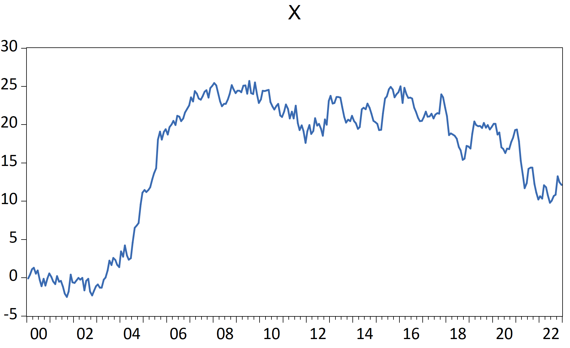
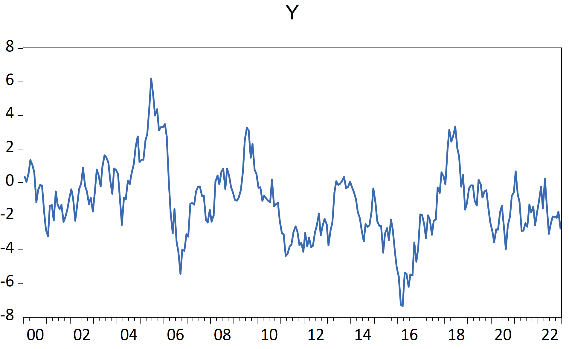
Figure 7.1: EViews graphs imported automatically by fig-EviewsR chunk
The above chunk creates an Eviews program with the chunk’s content,
then automatically open Eviews and run the program, which will create an
Eviews workfile with pages containing monthly sample from 2000 to 2022.
The program will also save an EViews workfile named
EviewsR_workfile in the current directory.
The eviews chunk automatically returns the outputs of
each equation object as a dataframe, accessible via
chunkLabel$pageName_equationName. For example, The
R2 of the ols equation object is
0.044951, which can be accessed using
`r EviewsR$eviewsrpage_ols$r2`. We can obtain the table
object by chunkLabel$pageName_tableName. Therefore,
EviewsR$eviewsrpage_olstable will give us the
OLSTable object as dataframe. Note the underscore
(_) between the pageName and
equationName, and between the pageName and
tableName.
EviewsR$eviewsrpage_ols$r2
#> [1] 0.044951
EviewsR$eviewsrpage_ols$aic
#> [1] 4.310163
K = EviewsR$eviewsrpage_olstable[c(6, 8, 9), 1:5]
colnames(K) = NULL
knitr::kable(K, row.names = F, caption = "Selected cells of EViews table object")| Variable | Coefficient | Std. Error | t-Statistic | Prob. |
| C | -0.301413 | 0.260956 | -1.155033 | 0.2491 |
| X | -0.051410 | 0.014316 | -3.591137 | 0.0004 |
Table 7.1: Selected cells of EViews table object
The EViews series objects are also imported automatically as
dataframe (by default) or xts objects (if we use chunk
option class="xts"). They are accessed via
chunkLabel$pageName.
EviewsR$eviewsrpage %>%
    head()
#>         date           x          y
#> 1 2000-01-01 -0.06062345 0.34705763
#> 2 2000-02-01  0.40287977 0.04959103
#> 3 2000-03-01  1.13387526 0.56589164
#> 4 2000-04-01  1.34089330 1.35264827
#> 5 2000-05-01  0.54596099 1.05434874
#> 6 2000-06-01 0.96869514 0.61693341The function create_object() can be used to create an
Eviews object in the existing EViews workfile.
create_object(wf = "EviewsR_workfile", action = "equation", action_opt = "",
    object_name = "eviews_equation", view_or_proc = "ls", options_list = "",
    arg_list = "y ar(1)")

create_object(wf = "EviewsR_workfile", object_name = "x1", object_type = "series",
expression = "y^2")EViews graphs can be included in R Markdown or Quarto document by
eviews_graph() function.
To create graph from existing EViews series objects:
eviews_graph(wf = "EviewsR_workfile", page = "EviewsRPage", series = "x y",
    mode = "overwrite", graph_procs = "setelem(1) lcolor(red) lwidth(4)",
    graph_options = "m")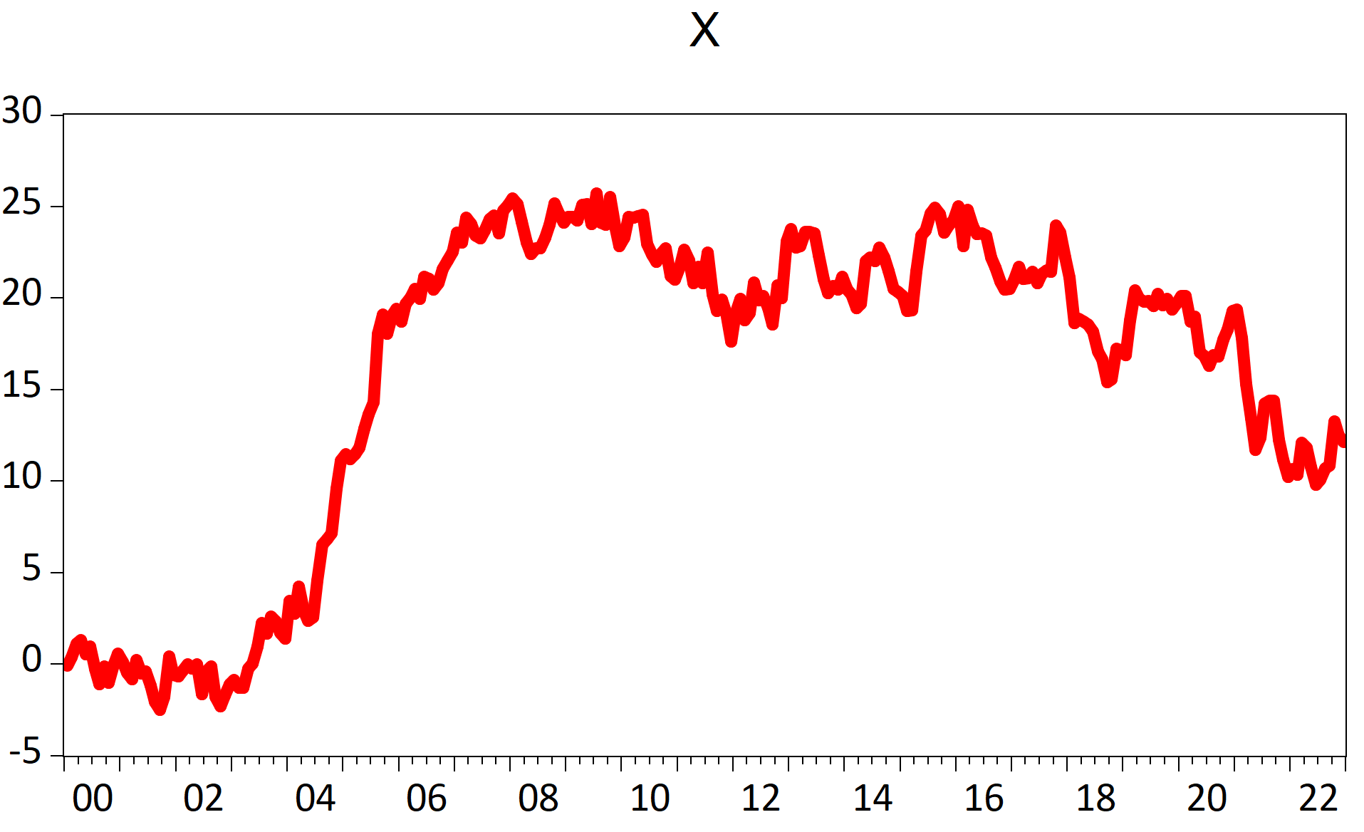
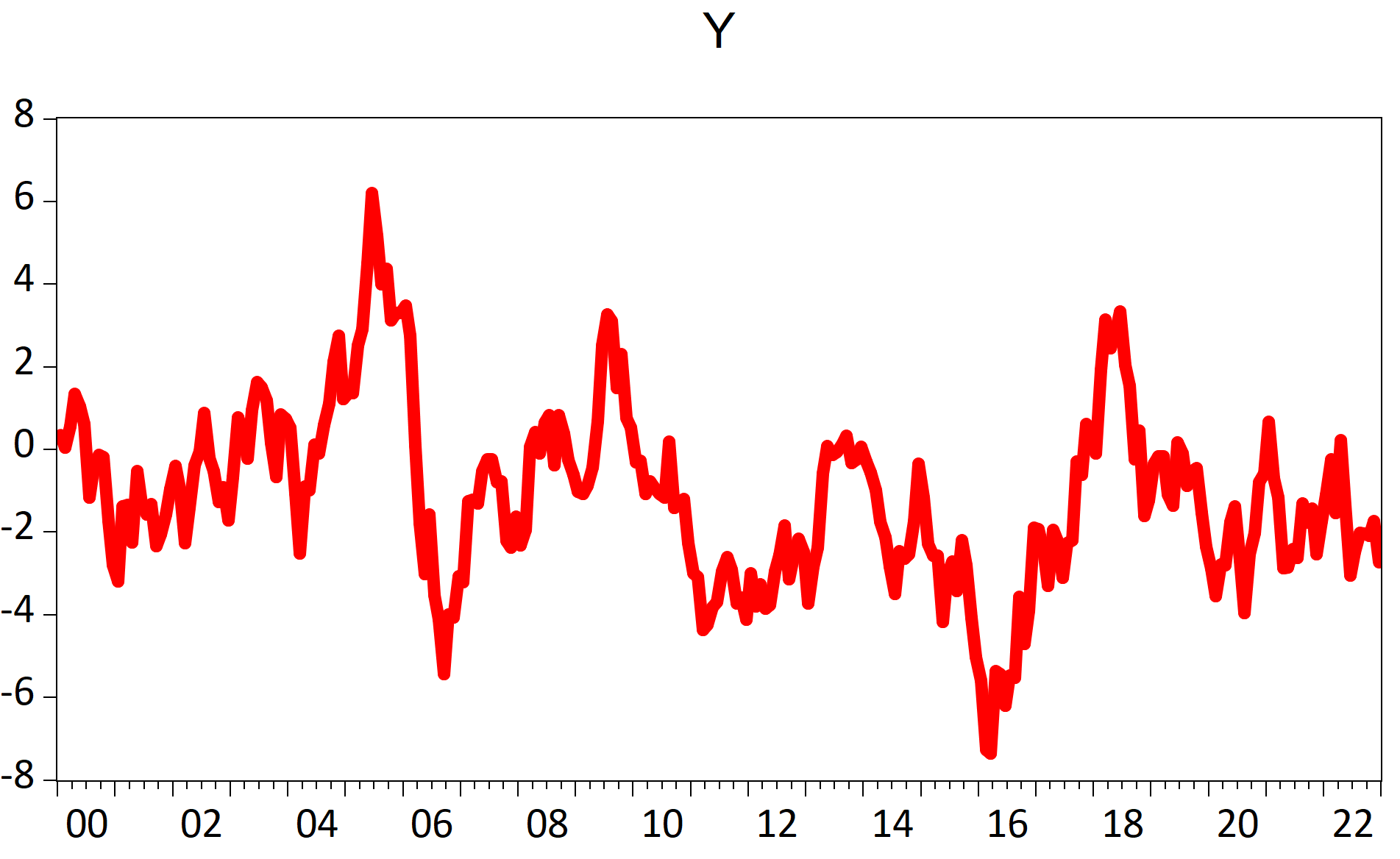
Figure 7.2: Graphs of existing EViews series objects imported by fig-eviewsGraph chunk
We can also create graph objects from an R dataframe
Data = data.frame(x = cumsum(rnorm(100)), y = cumsum(rnorm(100)))
eviews_graph(series = Data, group = TRUE, start_date = "1990Q4",
    frequency = "Q")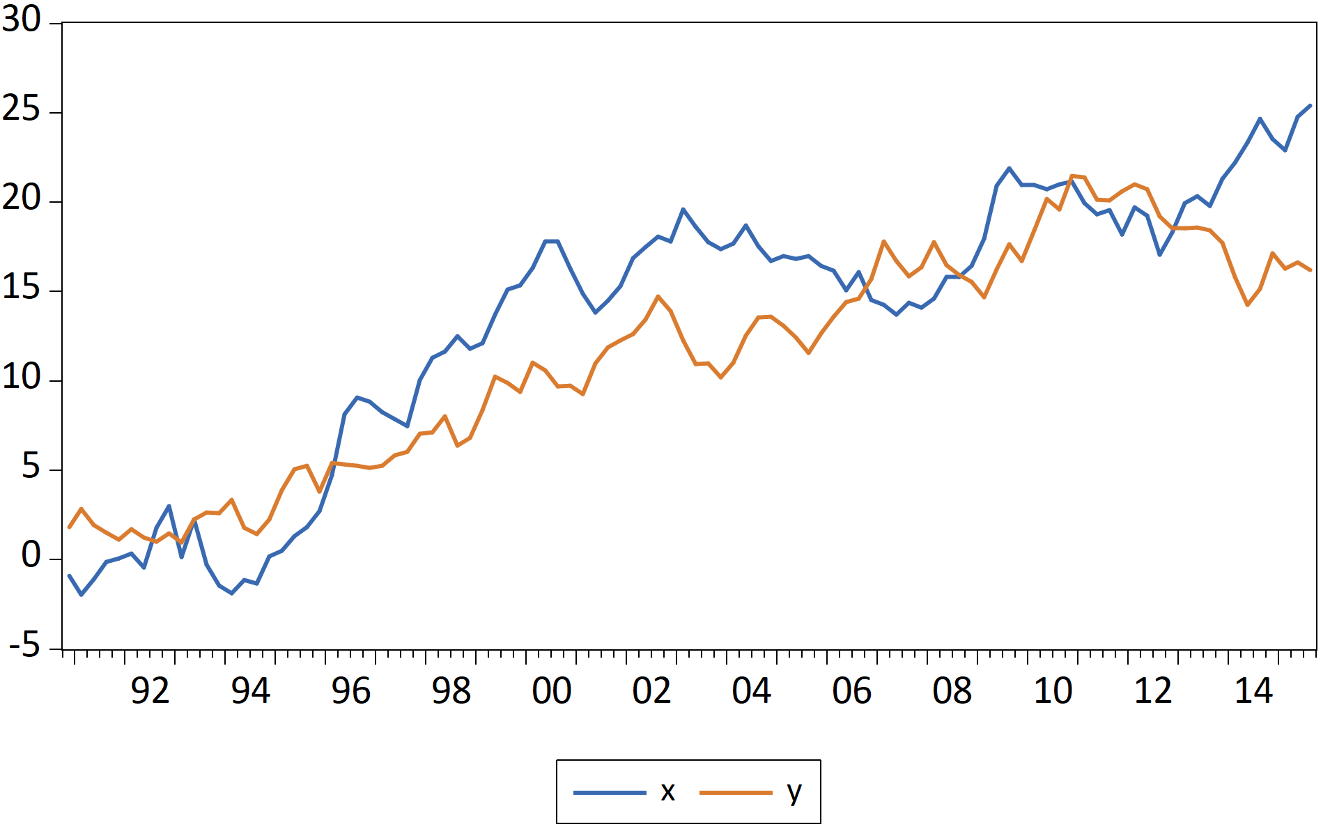
Figure 7.3: Graphs of an R dataframe imported by fig-eviewsGraph1 chunk
To plot a scatter graph and histogram on the same frame:
eviews_graph(wf = "EviewsR_workfile", page = "EviewsRPage", series = "x y",
    group = T, graph_command = "scat(ab=histogram) linefit()",
    mode = "overwrite", graph_procs = "setelem(1) lcolor(green) lwidth(2)")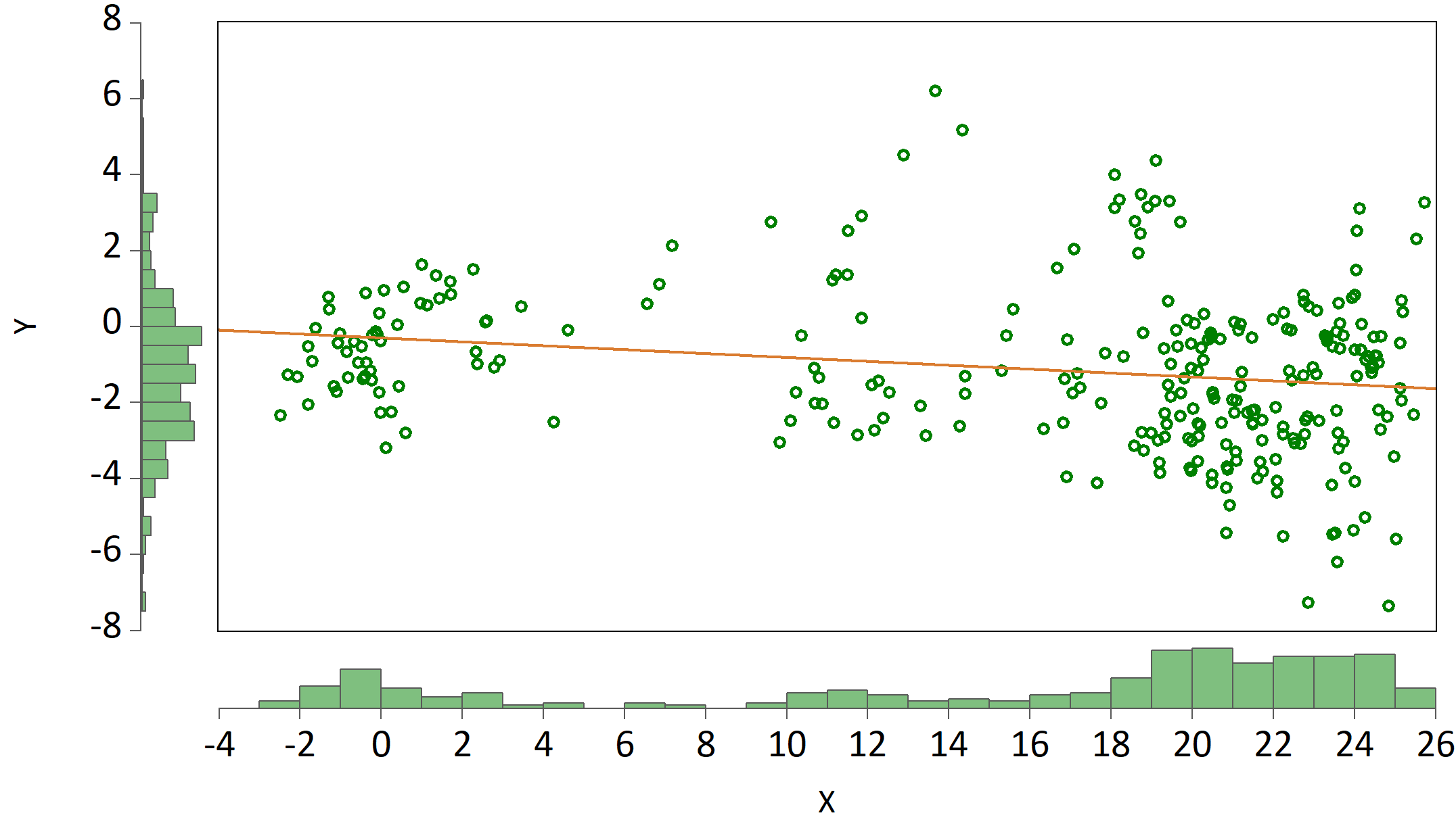
Figure 7.4: Scatter graph along with histogram
Data can be imported from external sources by
eviews_import() function.
eviews_import(source_description = "eviews_import.csv", start_date = "1990",
    frequency = "m", rename_string = "x ab", smpl_string = "1990m10 1992m10")
Alternatively, use the dataframe as the
source_description.
eviews_import(source_description = Data, wf = "eviews_import1",
    start_date = "1990", frequency = "m", rename_string = "x ab",
smpl_string = "1990m10 1992m10")Similar to Eviews workfile, an Eviews page can be saved in various
formats by eviews_pagesave() function.
eviews_pagesave(wf = "eviewsr_workfile", page = "EviewsRPage",
source_description = "pagesave.csv", drop_list = "y")An Eviews workfile can be created using
eviews_wfcreate() function in R.
eviews_wfcreate(wf = "eviews_wfcreate", page = "EviewsRPage",
    frequency = "m", start_date = "1990", end_date = "2022")
Create a workfile from a dataframe
eviews_wfcreate(source_description = Data, wf = "eviews_wfcreate1",
page = "EviewsR_page", frequency = "m", start_date = "1990")An EViews workfile can be saved various output formats using
eviews_wfsave() in function in R.
eviews_wfsave(wf = "eviewsr_workfile", source_description = "wfsave.csv")A set of Eviews commands can be executed with the help of
exec_commands() function in R.
exec_commands(c("wfcreate(wf=exec_commands,page=eviewsPage) m 2000 2022"))

eviewsCommands = "pagecreate(page=eviewspage1) 7 2020 2022
for %page eviewspage eviewspage1
pageselect {%page}
genr y=@cumsum(nrnd)
genr x=@cumsum(nrnd)
equation ols.ls y c x
graph x_graph.line x
graph y_graph.area y
freeze(OLSTable,mode=overwrite) ols
next"
exec_commands(commands = eviewsCommands, wf = "exec_commands")Use export_dataframe() function to export dataframe
object to Eviews.
export_dataframe(wf = "export_dataframe", source_description = Data,
start_date = "1990", frequency = "m")Import EViews equation data members into R, R Markdown or Quarto.
import_equation(wf = "EviewsR_workfile", page = "EviewsRPage",
    equation = "OLS")
To access the imported equation in base R:
Import EViews graph objects(s) into R, R Markdown or Quarto.
import_graph(wf = "eviewsr_workfile")

Figure 7.5: EViews graphs imported using import_graph() function
To import only graphs that begin with x:
import_graph(wf = "exec_commands", graph = "x*")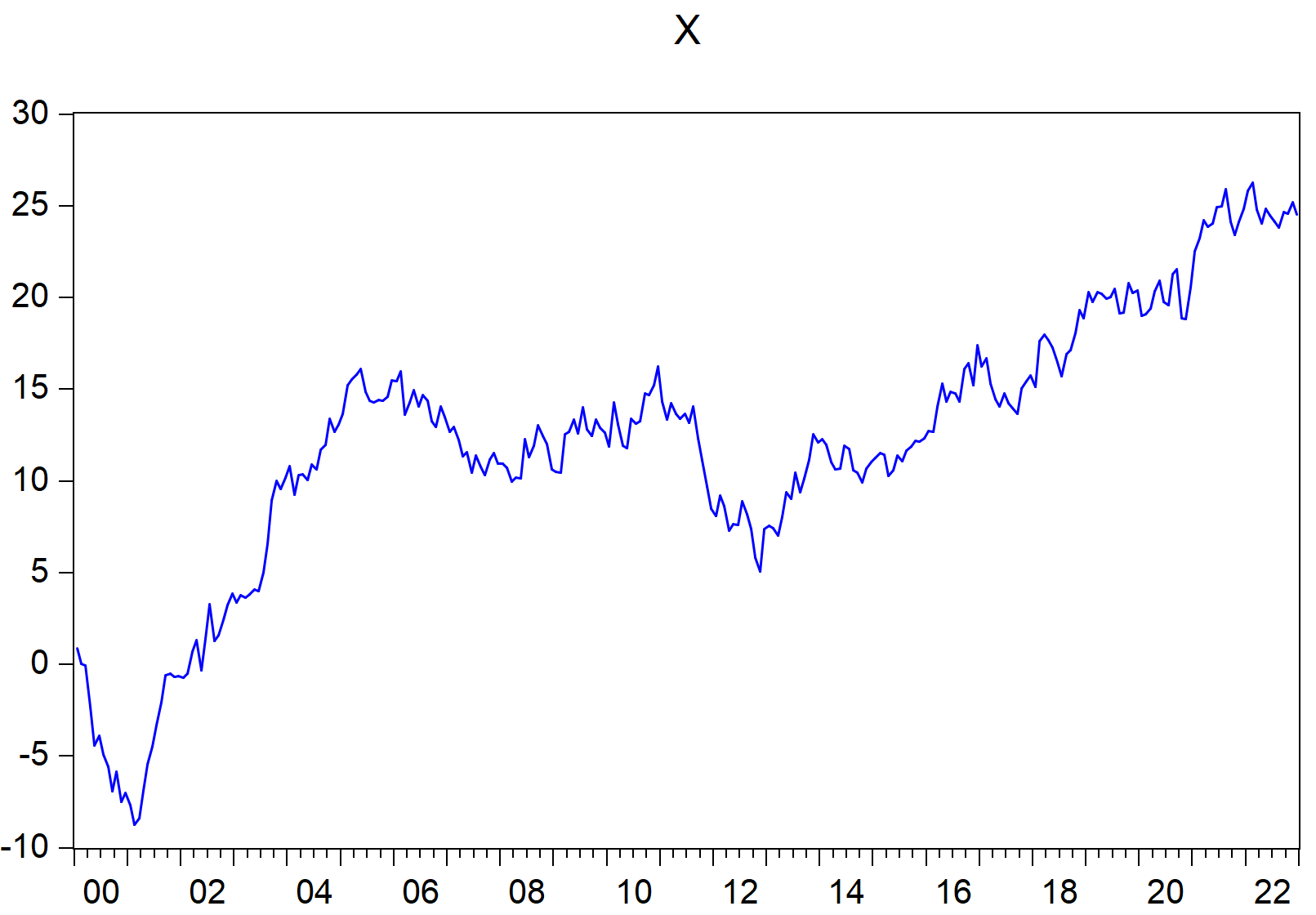
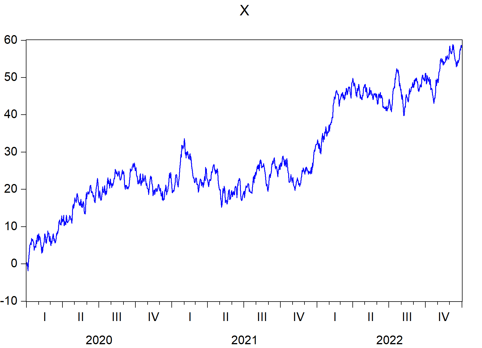
Figure 7.6: EViews graphs that begin with X imported using import_graph() function
Eviews tables can be imported as kable object by
import_kable() function. Therefore, we can include the
import_kable(wf = "EViewsR_workfile", page = "EviewsRPage", table = "OLSTable",
    format = "html", caption = "Selected cells of EViews table imported using import_kable() function",
range = "r7c1:r10c5", digits = 3)| Variable | Coefficient | Std. Error | t-Statistic | Prob. |
|---|---|---|---|---|
| C | -0.301 | 0.261 | -1.155 | 0.249 |
| X | -0.051 | 0.014 | -3.591 | 0.000 |
Use import_series() function to import data from EViews
to R as a dataframe. The function creates a new environment
eviews, whose objects can be accessed via
eviews$pageName.
import_series(wf = "eviewsr_workfile")To access the series in base R:
eviews$eviewspage %>%
    head()
To import the series as an xts object:
import_series(wf = "eviewsr_workfile", series = c("x", "y"),
class = "xts")Import EViews table objects(s) into R, R Markdown or Quarto.
To import all table objects across all pages
import_table(wf = "EviewsR_workfile")To import specific table objects, for example
OLSTable
import_table(wf = "EviewsR_workfile", table = "OLStable")To import table objects on specific pages
import_table(wf = "EviewsR_workfile", page = " EviewsRPage")To access the table in base R
(eviews$pageName_tableName)
eviews$eviewspage_olstableImport EViews equation data members, graph, series and table
objects(s) into R, R Markdown or Quarto. This function is a blend of
import_equation(), import_graph(),
import_series() and import_table()
functions.
To import all equation, graph, series and table objects across all pages
import_workfile(wf = "EviewsR_workfile")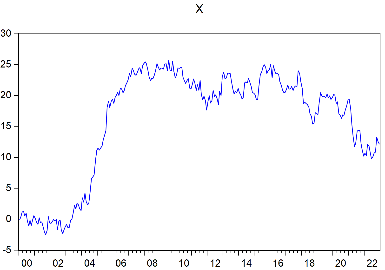
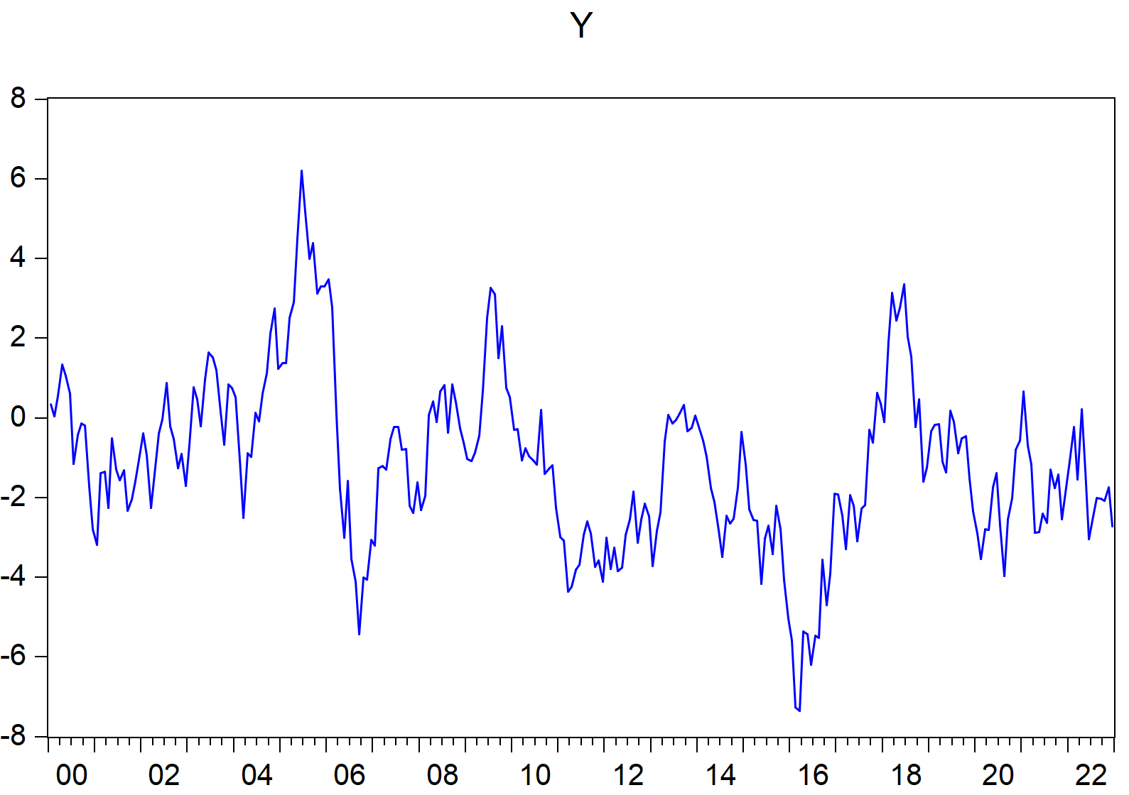
Figure 7.7: EViews graphs automatically imported by import_workfile() function
To import specific objects
import_workfile(wf = "exec_commands", equation = "ols", graph = "x*",
    series = "y*", table = "ols*")
To import objects on specific page(s)
import_workfile(wf = "exec_commands", page = "eviewspage eviewspage1")To access the objects in base R:
eviews$eviewspage_ols  # equation
# eviewspage-x_graph # graph saved in 'figure/' folder
eviews$eviewspage %>%
    head()  # series
eviews$eviewspage_olstable # tableA set of random walk series can be simulated in R using EViews
engine, thanks to rwalk() function.
rwalk(wf = "eviewsr_workfile", series = "X Y Z", page = "", rndseed = 12345,
    frequency = "M", num_observations = 100, class = "xts")

xts::plot.xts(rwalk$xyz, type = "l", main = "")
ggplot2::autoplot(rwalk$xyz, facet = "")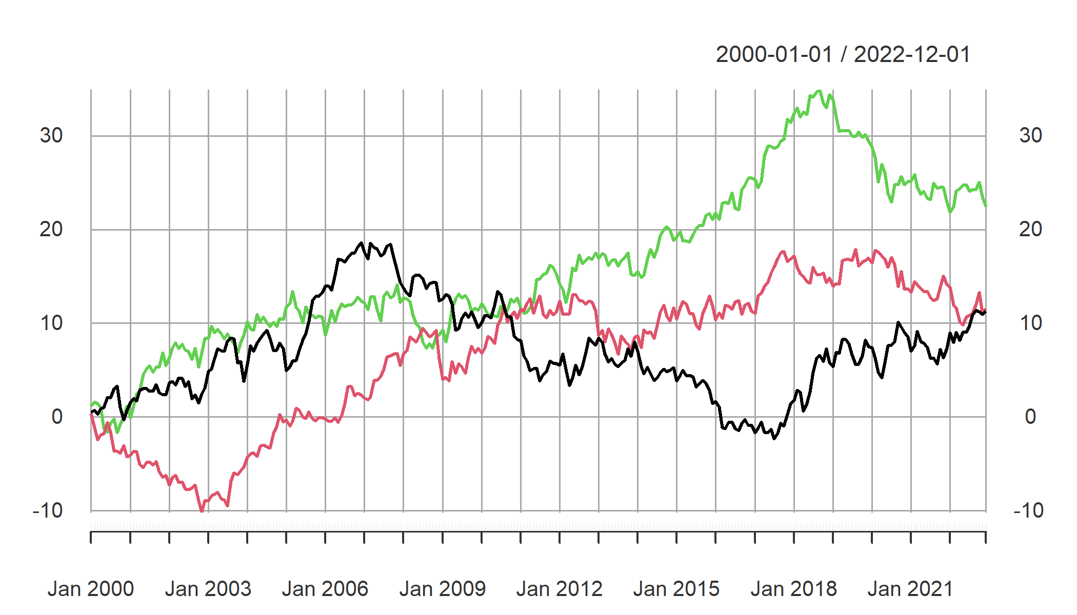
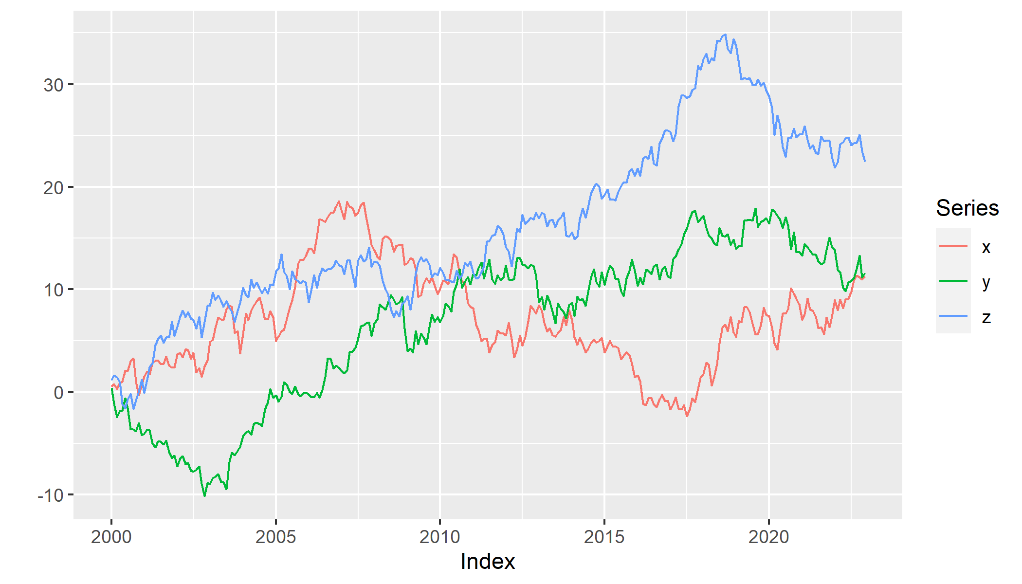
Figure 7.8: Plots of imported EViews random walk series objects
The demo files are included and can be accessed via
demo(package="EviewsR")
demo(create_object())
demo(eviews_graph())
demo(eviews_import())
demo(eviews_pagesave())
demo(eviews_wfcreate())
demo(eviews_wfsave())
demo(exec_commands())
demo(export_dataframe())
demo(import_equation())
demo(import_graph())
demo(import_kable())
demo(import_series())
demo(import_table())
demo(import_workfile())
demo(rwalk())
demo(set_eviews_path())Template for R Markdown is created. Go to
file->New File->R Markdown-> From Template->EviewsR.
You might be interested in the following packages:
Please download the example files from Github.