This package is grounded in a branch of spatial statistics. Using
geographically weights, the geographically weighted panel regression is
try to solve the residuals from panel regression clustering spatially.
To investigate whether the residuals cluster spatially, the Moran’s I
test is also improved. Furthermore, three local statistic tests are
contained to help the users select model.
This package includes the function for the optimal bandwidth selection
in GWPR, the function for GWPR, the function for the local Hausman test,
the function for the local F test for individual effects, the function
for the local Lagrange Multiplier Breusch-Pagan test, and the function
for panel Moran’s I test. The functions have been optimized, which
require the less memory in the calculation.
Chao Li chaoli0394@gmail.com Shunsuke Managi managi@doc.kyushu-u.ac.jp
Chao Li chaoli0394@gmail.com
You can install the released version of GWPR.light from CRAN with:
install.packages("GWPR.light")You can read our vignettes
This is a basic example which shows you how to solve a common problem:
library(GWPR.light)library(tmap)
## basic example code
data(TransAirPolCalif)
data(California)
formula.GWPR <- pm25 ~ co2_mean + Developed_Open_Space_perc + Developed_Low_Intensity_perc +
Developed_Medium_Intensity_perc + Developed_High_Intensity_perc +
Open_Water_perc + Woody_Wetlands_perc + Emergent_Herbaceous_Wetlands_perc +
Deciduous_Forest_perc + Evergreen_Forest_perc + Mixed_Forest_perc +
Shrub_perc + Grassland_perc + Pasture_perc + Cultivated_Crops_perc +
pop_density + summer_tmmx + winter_tmmx + summer_rmax + winter_rmaxThis is an example about GWPR.moran.test:
pdata <- plm::pdata.frame(TransAirPolCalif, index = c("GEOID", "year"))
moran.plm.model <- plm::plm(formula = formula.GWPR, data = pdata, model = "within")
#summary(moran.plm.model)

bw.AIC.F <- bw.GWPR(formula = formula.GWPR, data = TransAirPolCalif, index = c("GEOID", "year"), SDF = California,
                     adaptive = F, p = 2, bigdata = F, effect = "individual",
                     model = "within", approach = "AIC", kernel = "bisquare", longlat = F,
                     doParallel = T, cluster.number = 4)
#> To make sure every subsample have enough freedom, the minimun numbers of individuals is 2
#> The upper boundary is 12.2397827722445, and the lower boudnary is 1.4354355959204
#> ..................................................................................
#> You use parallel process, so be careful about your memory usage. Cluster number: 4
#> Fixed Bandwidth: 8.112889 AIC score: 2468.518
#> Fixed Bandwidth: 5.562329 AIC score: 1993.051
#> Fixed Bandwidth: 3.985996 AIC score: 1507.388
#> Fixed Bandwidth: 3.011769 AIC score: 1098.755
#> Fixed Bandwidth: 2.409663 AIC score: 802.8273
#> Fixed Bandwidth: 2.037541 AIC score: 613.6641
#> Fixed Bandwidth: 1.807557 AIC score: Inf
#> Fixed Bandwidth: 2.179679 AIC score: 680.1113
#> Fixed Bandwidth: 1.949695 AIC score: Inf
#> Fixed Bandwidth: 2.091833 AIC score: 640.8903
#> Fixed Bandwidth: 2.003987 AIC score: Inf
#> Fixed Bandwidth: 2.058279 AIC score: 623.5577
#> Fixed Bandwidth: 2.024725 AIC score: 607.2684
#> Fixed Bandwidth: 2.016804 AIC score: 604.0248
#> Fixed Bandwidth: 2.011908 AIC score: 601.4765
#> Fixed Bandwidth: 2.008883 AIC score: Inf
#> Fixed Bandwidth: 2.013778 AIC score: 602.001
#> Fixed Bandwidth: 2.010752 AIC score: 601.1515
#> Fixed Bandwidth: 2.010038 AIC score: Inf
#> Fixed Bandwidth: 2.011194 AIC score: 601.2757
#> Fixed Bandwidth: 2.01048 AIC score: Inf
#> Fixed Bandwidth: 2.010921 AIC score: 601.199
#> Fixed Bandwidth: 2.010648 AIC score: 601.1222
#> Fixed Bandwidth: 2.010584 AIC score: 601.1041
#> Fixed Bandwidth: 2.010544 AIC score: 601.0928
#> Fixed Bandwidth: 2.010519 AIC score: Inf
#> Fixed Bandwidth: 2.010559 AIC score: 601.0971
#> Fixed Bandwidth: 2.010535 AIC score: 601.0902
#> Fixed Bandwidth: 2.010529 AIC score: 601.0886

# moran's I test
GWPR.moran.test(moran.plm.model, SDF = California, bw = bw.AIC.F, kernel = "bisquare",
                 adaptive = F, p = 2, longlat=F, alternative = "greater")
#> $statistic
#> [1] 3.174358
#>
#> $p.value
#> [1] 0.0007508427
#>
#> $Estimated.I
#> [1] 0.002129923
#>
#> $Excepted.I
#> [1] -0.01754386
#>
#> $V2
#> [1] 3.841174e-05
#>
#> $alternative
#> [1] "greater"
# The statistic is significantly greater than 0. Therefore, the residuals are spatially clustered.
GWPR example:
result.F.AIC <- GWPR(bw = bw.AIC.F, formula = formula.GWPR, data = TransAirPolCalif, index = c("GEOID", "year"),
                     SDF = California, adaptive = F, p = 2, effect = "individual", model = "within",
                     kernel = "bisquare", longlat = F)
#> ************************ GWPR Begin *************************
#> Formula: pm25  =  co2_mean + Developed_Open_Space_perc + Developed_Low_Intensity_perc + Developed_Medium_Intensity_perc + Developed_High_Intensity_perc + Open_Water_perc + Woody_Wetlands_perc + Emergent_Herbaceous_Wetlands_perc + Deciduous_Forest_perc + Evergreen_Forest_perc + Mixed_Forest_perc + Shrub_perc + Grassland_perc + Pasture_perc + Cultivated_Crops_perc + pop_density + summer_tmmx + winter_tmmx + summer_rmax + winter_rmax -- Individuals: 58
#> Bandwidth: 2.01052881685978 ---- Adaptive: FALSE
#> Model: within ---- Effect: individual
#> The R2 is: 0.896960603213274
#> Note: in order to avoid mistakes, we forced a rename of the individuals'ID as "id".
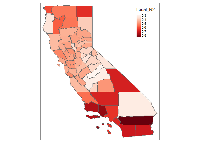
summary(result.F.AIC$SDF$Local_R2)
#>    Min. 1st Qu.  Median    Mean 3rd Qu.    Max.
#>  0.2899  0.4272  0.4676  0.4928  0.5375  0.8467
tm_shape(result.F.AIC$SDF) +
  tm_polygons(col = "Local_R2", pal = "Reds",auto.palette.mapping = F,
              style = 'cont')
#> Warning: The argument auto.palette.mapping is deprecated. Please use midpoint
#> for numeric data and stretch.palette for categorical data to control the palette
#> mapping.
#> Warning in sp::proj4string(obj): CRS object has comment, which is lost in output
#> Linking to GEOS 3.9.0, GDAL 3.2.1, PROJ 7.2.1
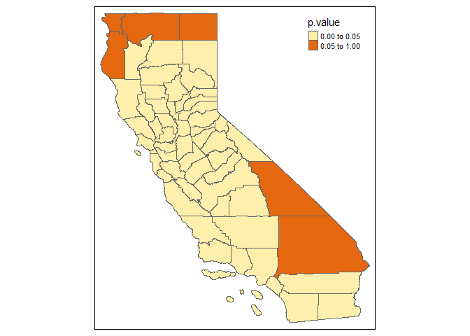
Example of F test:
GWPR.pFtest.resu.F <- GWPR.pFtest(formula = formula.GWPR, data = TransAirPolCalif, index = c("GEOID", "year"),
                                  SDF = California, bw = bw.AIC.F, adaptive = F, p = 2, effect = "individual",
                                  kernel = "bisquare", longlat = F)
#> **************************** F test in each subsample *********************************
#> Formula: pm25  =  co2_mean + Developed_Open_Space_perc + Developed_Low_Intensity_perc + Developed_Medium_Intensity_perc + Developed_High_Intensity_perc + Open_Water_perc + Woody_Wetlands_perc + Emergent_Herbaceous_Wetlands_perc + Deciduous_Forest_perc + Evergreen_Forest_perc + Mixed_Forest_perc + Shrub_perc + Grassland_perc + Pasture_perc + Cultivated_Crops_perc + pop_density + summer_tmmx + winter_tmmx + summer_rmax + winter_rmax -- Individuals: 58
#> Bandwidth:2.01052881685978 ---- Adaptive: FALSE
#> Model: Fixed Effects vs Pooling ---- Effect: individual
#> If the p-value is lower than the specific level (0.01, 0.05, etc.), significant effects exist.
tm_shape(GWPR.pFtest.resu.F$SDF) +
     tm_polygons(col = "p.value", breaks = c(0, 0.05, 1))
#> Warning in sp::proj4string(obj): CRS object has comment, which is lost in output
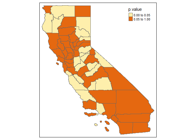
Example of Locally Breusch-Pagan Lagrange Multiplier Test:
GWPR.plmtest.resu.F <- GWPR.plmtest(formula = formula.GWPR, data = TransAirPolCalif, index = c("GEOID", "year"),
                                    SDF = California, bw = bw.AIC.F, adaptive = F, p = 2,
                                    kernel = "bisquare", longlat = F)
#> **************** Breusch-Pagan Lagrange Multiplier test in each subsample *******************
#> Formula: pm25  =  co2_mean + Developed_Open_Space_perc + Developed_Low_Intensity_perc + Developed_Medium_Intensity_perc + Developed_High_Intensity_perc + Open_Water_perc + Woody_Wetlands_perc + Emergent_Herbaceous_Wetlands_perc + Deciduous_Forest_perc + Evergreen_Forest_perc + Mixed_Forest_perc + Shrub_perc + Grassland_perc + Pasture_perc + Cultivated_Crops_perc + pop_density + summer_tmmx + winter_tmmx + summer_rmax + winter_rmax -- Individuals: 58
#> Bandwidth: 2.01052881685978 ---- Adaptive: FALSE
#> Model: Pooling ----
#> If the p-value is lower than the specific level (0.01, 0.05, etc.), significant effects exist.
tm_shape(GWPR.plmtest.resu.F$SDF) +
     tm_polygons(col = "p.value", breaks = c(0, 0.05, 1))
#> Warning in sp::proj4string(obj): CRS object has comment, which is lost in output
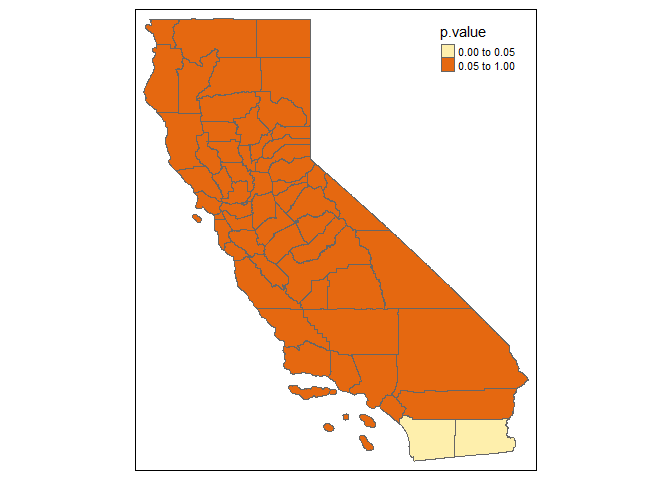
Example of Locally Hausman Test Based on GWPR
GWPR.phtest.resu.F <- GWPR.phtest(formula = formula.GWPR, data = TransAirPolCalif, index = c("GEOID", "year"),
                                  SDF = California, bw = bw.AIC.F, adaptive = F, p = 2, effect = "individual",
                                  kernel = "bisquare", longlat = F, random.method = "amemiya")
#> ************************* Hausman Test in each subsample ***************************
#> Formula: pm25  =  co2_mean + Developed_Open_Space_perc + Developed_Low_Intensity_perc + Developed_Medium_Intensity_perc + Developed_High_Intensity_perc + Open_Water_perc + Woody_Wetlands_perc + Emergent_Herbaceous_Wetlands_perc + Deciduous_Forest_perc + Evergreen_Forest_perc + Mixed_Forest_perc + Shrub_perc + Grassland_perc + Pasture_perc + Cultivated_Crops_perc + pop_density + summer_tmmx + winter_tmmx + summer_rmax + winter_rmax -- Individuals: 58
#> Bandwidth: 2.01052881685978 ---- Adaptive: FALSE
#> Model: Fixed Effects vs Random Effects ---- Effect: individual ---- Random Method: amemiya
#> If the p-value is lower than the specific level (0.01, 0.05, etc.), one model is inconsistent.
tm_shape(GWPR.phtest.resu.F$SDF) +
     tm_polygons(col = "p.value", breaks = c(0, 0.05, 1))
#> Warning in sp::proj4string(obj): CRS object has comment, which is lost in output