GauPro

Overview

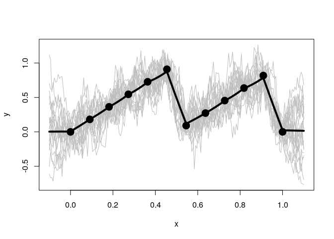
This package allows you to fit a Gaussian process to a dataset. A Gaussian process is a commonly used model in computer simulation. It assumes that the distribution of any set of points is multivariate normal with a constant mean and a correlation function.

The newest release allows you to use different kernel and trend functions, instead of just a squared exponential covariance.

You should probably use a different package for your modeling, such as laGP, mlegp, or GPfit if you are using R, or GPy if you are using Python.

Installation

You can install like any other package

install.packages('GauPro')

The most up-to-date version can be downloaded from my Github account.

# install.packages("devtools")
devtools::install_github("CollinErickson/GauPro")

Examples in 1-Dimension

Fit a sine curve with noise.

n <- 12
x <- matrix(seq(0,1,length.out = n), ncol=1)
y <- sin(2*pi*x) + rnorm(n,0,1e-1)
gp <- GauPro::GauPro(X=x, Z=y)
curve(gp$pred(x));points(x,y)
curve(gp$pred(x)+2*gp$pred(x,T)$se,col=2,add=T);curve(gp$pred(x)-2*gp$pred(x,T)$se,col=2,add=T)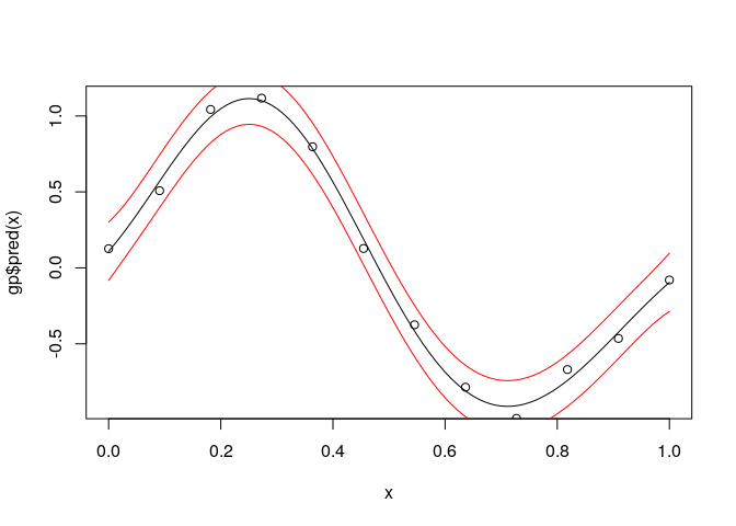

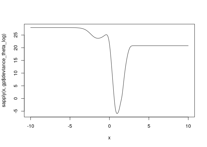
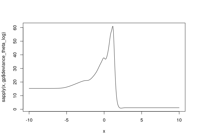
This is the likelihood as a function of the log of theta. It is not convex and is difficult to optimize in general.

curve(sapply(x, gp$deviance_theta_log),-10,10, n = 300) # deviance profile

Fit a sawtooth function with no noise.

n <- 12
x <- matrix(seq(0,1,length.out = n), ncol=1)
y <- (2*x) %%1
gp <- GauPro::GauPro(X=x, Z=y)
curve(gp$pred(x));points(x,y)
curve(gp$pred(x)+2*gp$pred(x,T)$se,col=2,add=T);curve(gp$pred(x)-2*gp$pred(x,T)$se,col=2,add=T)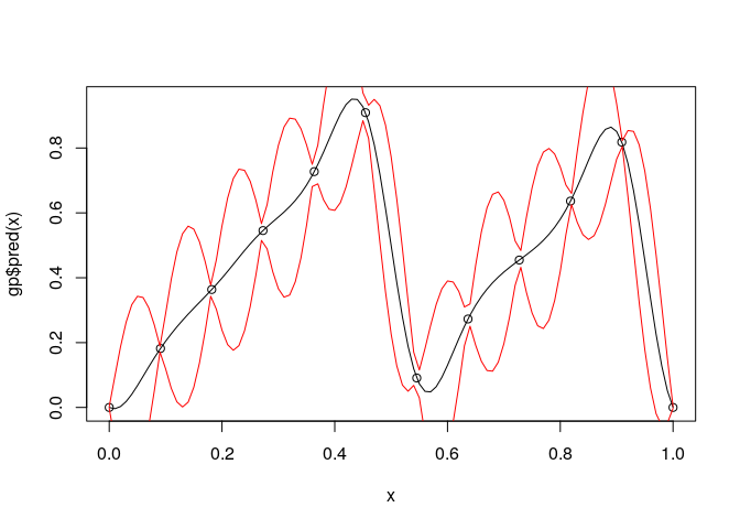

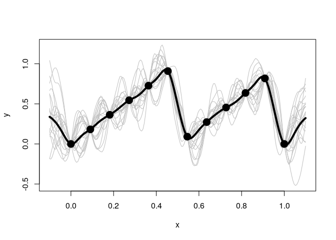
curve(sapply(x, gp$deviance_theta_log),-10,10, n = 300) # deviance profile

Using kernels

library(GauPro)

The kernel, or covariance function, has a large effect on the Gaussian process being estimated. The function GauPro uses the squared exponential, or Gaussian, covariance function. The newer version of GauPro has a new function that will fit a model using whichever kernel is specified.

To do this a kernel must be specified, then passed to GauPro_kernel_model$new. The example below shows what the Matern 5/2 kernel gives.

kern <- Matern52$new(0)
gpk <- GauPro_kernel_model$new(matrix(x, ncol=1), y, kernel=kern, parallel=FALSE)
if (requireNamespace("MASS", quietly = TRUE)) {
  plot(gpk)
}

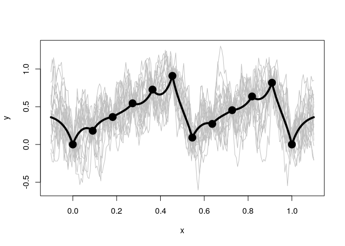
The exponential kernel is shown below. You can see that it has a huge effect on the model fit. The exponential kernel assumes the correlation between points dies off very quickly, so there is much more uncertainty and variation in the predictions and sample paths.

kern.exp <- Exponential$new(0)
gpk.exp <- GauPro_kernel_model$new(matrix(x, ncol=1), y, kernel=kern.exp, parallel=FALSE)
if (requireNamespace("MASS", quietly = TRUE)) {
  plot(gpk.exp)
}

Trends

Along with the kernel the trend can also be set. The trend determines what the mean of a point is without any information from the other points. I call it a trend instead of mean because I refer to the posterior mean as the mean, whereas the trend is the mean of the normal distribution. Currently the three options are to have a mean 0, a constant mean (default and recommended), or a linear model.

With the exponential kernel above we see some regression to the mean. Between points the prediction reverts towards the mean of 0.4006891. Also far away from any data the prediction will near this value.

Below when we use a mean of 0 we do not see this same reversion.

kern.exp <- Exponential$new(0)
trend.0 <- trend_0$new()
gpk.exp <- GauPro_kernel_model$new(matrix(x, ncol=1), y, kernel=kern.exp, trend=trend.0, parallel=FALSE)
if (requireNamespace("MASS", quietly = TRUE)) {
  plot(gpk.exp)
}