The Omitted Variable Tool (OVtool) package was designed to assess the sensitivity of research findings to omitted variables when estimating causal effects using propensity score (PS) weighting. This package includes graphics and summary results that will enable a researcher to quantify the impact an omitted variable would have on their results. Burgette et al. (2021) describe the methodology behind the primary function in this package, ov_sim(). This document presents syntax for the implementation of the ov_sim() function and provides an example of how to interpret the packages’ graphical output.
This package is useful in a wide range of applications where researchers want to analyze how sensitive their research findings are to unobserved confounders that were not included in their propensity score and outcome models. It will estimate the potential impact of the unobserved confounders on both the estimated treatment or exposure effects as well as on the statistical significance of an analysis.
This package is demonstrated using a synthetic data set that was derived from a large-scale observational study on youth in substance use treatment. More specifically, it contains a subset of measures from the Global Appraisal of Individual Needs (GAIN) biopsychosocial assessment instrument (Dennis, Titus et al. 2003) from sites that administered two different types of substance use disorder treatments (treatment “A” and treatment “B”). This data set represents 4,000 adolescents. The main goal of this analysis is to understand the relative effectiveness of Treatment A versus Treatment B on mental health outcomes and to assess the potential for an omitted variable to bias the findings. To create our synthetic data set, we used an R package called “synthpop : Bespoke Creation of Synthetic Data in R” (Nowok et al. 2016).
In our synthetic dataset, there are 2,000 adolescents in each treatment group, as indicated in the treat variable. Within this data set there are 28 variables on substance use disorder and mental health outcomes. Variables that end in _0, _3, and _6 were collected from interviews at baseline, 3-, and 6-months post-baseline, respectively.
For this tutorial we are interested in the mental health outcome, eps7p_3, emotional problem scale (eps) recorded at three months. In particular, we want to estimate the relative effectiveness of treatment A versus B on reducing emotional problems in youth. eps7p_3 ranges from zero to one, where higher values of EPS indicate more emotional problems. Past research has concluded there are many variables that may influence treatment assignment and an adolescents’ emotional problems (Griffin et al., 2020). We utilize a selection of these variables in our propensity score and outcome models and provide their definitions below.
We begin by loading the package. Note: installing OVtool may require a large number of other package installations if they are not already installed on your machine. We recommend using a fresh R session prior to installation.
We can load the synthetic dataset and make our treatment variable a binary indicator of 0’s and 1’s. The OVtool requires the user to specify the treatment indicator as a numeric vector of 1’s and 0’s, where 1 indicates the target treatment group.
The relevant variables in this analysis are:
Treatment indicator treat: treatment program, a binary indicator where 1 and 0 represent Treatment “A” and Treatment “B”, respectively.
Outcome of interest eps7p_3: emotional problem scale at 3-months, a continuous variable ranging from 0 to 1. Higher values represent more emotional problems.
eps7p_0: emotional problem scale at baseline, a continuous variable ranging from 0 to 1. Like the outcome, higher values represent more emotional problems.
sfs8p_0: substance frequency scale 8-item version at baseline, a continuous variable ranging from 0 to 77.5. Higher values represent more frequencies of substance use.
sati_0: substance abuse treatment index at baseline, a continuous variable ranging from 0 to 110. Higher values indicate prior involvement in substance use treatment.
ada_0: adjusted days abstinent at baseline, a continuous variable ranging from 0 to 90 days.
recov_0: indicates whether the adolescent was in recovery at baseline, where 1 is in recovery and 0 is not in recovery.
tss_0: traumatic stress scale at baseline, a continuous variable ranging from 0 to 13. Higher values indicate more problems related to memories of traumatic events.
dss9_0: depressive symptom scale at baseline, a continuous variable ranging from 0 to 9. Higher values indicate higher levels of depressive symptoms.
For additional details on these variables, please refer to Dennis et al. (2003).
In the next two sections we showcase how our method works with a continuous outcome and binary treatment indicator. In the first analysis, we focus on how to use the OVtool when estimating the average treatment effect (ATE) for the population. In the second, we focus on estimating the average treatment effect on the treated (ATT) population. Note: One can also use the OVtool to assess sensitivity of findings for binary outcomes. With a binary outcome, the OVtool utilizes residuals linear probability model using observed covariates to generate the empirical CDF. If the residuals contain many ties, other types of sensitivity analyses may be more appropriate.
The OVtool can either take a vector of weights estimated using any method or a propensity score (ps) object produced by TWANG (Ridgeway et al., 2021). The chunk of code below demonstrates how to specify your propensity score model and generate propensity score weights using the ps function from TWANG. If you already have a column of weights in your dataset, you can skip to step 2.
## Create Formula
my_formula = as.formula(treat ~ eps7p_0 + sfs8p_0 + sati_0 + ada_0 + recov_0 +
                          tss_0 + dss9_0)

## Get weights
# library(twang)
ps.twang <- twang::ps(my_formula, data = sud, estimand = 'ATE', booster = "gbm",
                      stop.method = "ks.max", verbose=F, ks.exact = T)
The following line of code produces a balance table that demonstrates TWANG does a reasonable job of balancing. There are additional diagnostics we could check to ensure we have sufficient balance, but we move on without diving in further because the purpose of this tutorial is to showcase OVtool. See Ridgeway et al. for further information on balance diagnostics.
#> $unw
#>          tx.mn  tx.sd  ct.mn  ct.sd std.eff.sz   stat     p    ks ks.pval
#> eps7p_0  0.256  0.196  0.219  0.192      0.187  5.937 0.000 0.103   0.000
#> sfs8p_0 11.253 13.134 10.571 12.162      0.054  1.703 0.089 0.045   0.032
#> sati_0   8.233 22.128  2.145 10.658      0.345 11.088 0.000 0.121   0.000
#> ada_0   48.748 33.400 54.236 32.454     -0.166 -5.271 0.000 0.081   0.000
#> recov_0  0.246  0.431  0.240  0.427      0.015  0.479 0.632 0.006   1.000
#> tss_0    2.277  3.525  1.924  3.115      0.106  3.365 0.001 0.043   0.050
#> dss9_0   2.750  2.604  2.638  2.492      0.044  1.390 0.165 0.023   0.666
#>
#> $ks.max.ATE
#>          tx.mn  tx.sd  ct.mn  ct.sd std.eff.sz   stat     p    ks ks.pval
#> eps7p_0  0.239  0.194  0.233  0.192      0.028  0.880 0.379 0.021   0.765
#> sfs8p_0 10.885 12.655 10.727 12.372      0.012  0.392 0.695 0.012   0.998
#> sati_0   5.345 17.937  4.198 15.691      0.065  1.797 0.072 0.023   0.662
#> ada_0   51.455 32.894 52.377 32.898     -0.028 -0.858 0.391 0.020   0.823
#> recov_0  0.248  0.432  0.238  0.426      0.023  0.716 0.474 0.010   1.000
#> tss_0    2.099  3.358  2.065  3.279      0.010  0.313 0.754 0.012   0.999
#> dss9_0   2.675  2.556  2.706  2.535     -0.012 -0.381 0.703 0.012   0.999
The last step needed prior to moving onto the specification of your outcome model is to attach the weights as a column in your dataset. We extract the weights produced from ps in the line below.
# Get weights (not needed if user inserts a ps object in OVtool::outcome_model)
sud$w_twang = ps.twang$w$ks.max.ATEThe next step is to estimate the observed treatment effect. The outcome_model function in OVtool automatically uses the svydesign and svyglm functions from the survey package in R (survey) and formats and returns a list of components that are needed throughout step 3.
There are two options the researcher can take to input the relevant information to get their outcome results using outcome_model().
ps.object from TWANG and a stop.method (e.g. "ks.max") ordata used, the column name representing the weights, weights, and the column name representing the treatment indicator, treatment.The analyst must also provide:
outcomemodel_covariatesestimand# Run Models -- first standardize outcome
sud$eps7p_3_std = sud$eps7p_3/sd(sud$eps7p_3)
# Run outcome model (function in OVtool that calls svyglm from survey)
results = outcome_model(ps_object = NULL,
stop.method = NULL,
data = sud,
weights = "w_twang",
treatment = "treat",
outcome = "eps7p_3_std",
model_covariates = c("eps7p_0", "sfs8p_0",
"sati_0", "ada_0",
"recov_0", "tss_0",
"dss9_0"),
estimand = "ATE")
summary(results$mod_results)#>
#> Call:
#> svyglm(formula = formula, design = design_u)
#>
#> Survey design:
#> design_u <- survey::svydesign(ids=~1, weights=~w_orig, data=data)
#>
#> Coefficients:
#> Estimate Std. Error t value Pr(>|t|)
#> (Intercept) 0.4235011 0.0657531 6.441 1.33e-10 ***
#> treat 0.0712001 0.0278454 2.557 0.0106 *
#> eps7p_0 1.7397954 0.1166266 14.918 < 2e-16 ***
#> sfs8p_0 0.0015028 0.0020843 0.721 0.4709
#> sati_0 0.0028393 0.0012348 2.299 0.0215 *
#> ada_0 -0.0005808 0.0007725 -0.752 0.4522
#> recov_0 -0.0704673 0.0317912 -2.217 0.0267 *
#> tss_0 0.0329637 0.0069454 4.746 2.15e-06 ***
#> dss9_0 0.0540816 0.0080153 6.747 1.72e-11 ***
#> ---
#> Signif. codes: 0 '***' 0.001 '**' 0.01 '*' 0.05 '.' 0.1 ' ' 1
#>
#> (Dispersion parameter for gaussian family taken to be 0.7074412)
#>
#> Number of Fisher Scoring iterations: 2The outcome model results show an adjusted treatment effect estimate that accounts for confounding from observed covariates between youth in the two treatment programs (A = 1 and B = 0). From the results, we observe that the estimated treatment effect is 0.07 (p = 0.011), whereby youth receiving treatment A have slightly higher emotional problems at the 3-month follow-up than youth in treatment program B.
At this stage, researchers may ask themselves if the observed effect in Step 2 is real and how sensitive to unobserved confounders it is. Our tool is used to help answer this logical next step question.
The following snippet of code presents the main function in OVtool: ov_sim(). This function requires results from outcome_model() plus additional parameters including:
plot_covariates: a vector of column names potentially representing the covariates used to produce the analysts’ propensity score weights (these may or may not be the same as the list of covariates used for the outcome model)
es_grid: a vector on an effect size scale representing the range of association between the unobserved confounder (omitted variable) and the treatment indicator over which to run the simulations.
rho_grid: a vector of absolute correlations to simulate over. These correlations represent the range of absolute correlations between the omitted variable and the outcome
n_reps: the number of repetitions represents the number of times an unobserved confounder is simulated at each effect size and rho combination. The package defaults to 50. We find that fifty repetitions is sufficient in most cases, but the analyst may need to increase the number of repetitions if the plotted contours are not sufficiently smooth.
Optional arguments include:
progress: whether or not the function progress should print to screen. The default value is TRUE. If the user does not want the output to print to the console, they should set this parameter to FALSE.
add: The default value is FALSE. This is only set to TRUE if the user is running additional repetitions after the first call to ov_sim. It should be used if the original value of n_reps does not yield smooth contours.
sim_archive: The default value is NULL and is only used if add_reps is called. This parameter should never be defined by the user.
The ov_sim function does not require the user to specify vectors for es_grid and rho_grid. If the user specifies NULL for both, the tool will automatically suggest appropriate values. We define an effect size value in es_grid to show the strength of the relationship between the simulated unobserved covariate (U) and the treatment group indicator; it is defined as the standardized mean difference in U for the treatment A and treatment B groups. Typical rules of thumb for effect sizes (Cohen’s D) follow such that effect sizes greater than 0.2 would be considered small, 0.5 would be moderate and 0.8 would be large (Cohen, J., 1988). We define a particular value of rho specified in rho_grid as the absolute correlation the unobserved covariate (U) has with the outcome of interest, with larger values indicating stronger relationships between U and the outcome.
Please see Burgette et al. (2021) for additional details on the theory behind OVtool.
# Run OVtool (with weights (not a ps object))
ovtool_results_twang = ov_sim(model_results=results,
                              plot_covariates=c("eps7p_0", "sfs8p_0",
                                                "sati_0", "ada_0",
                                                "recov_0", "tss_0",
                                                "dss9_0"),
                              es_grid = NULL,
                              rho_grid = seq(0, 0.40, by = 0.05),
                              n_reps = 50,
                              progress = TRUE,
                              add = FALSE,
                              sim_archive = NULL)
The grid values are not required; if es_grid and/or rho_grid are set to NULL, the tool will calculate reasonable values to simulate over. For this tutorial we set es_grid to NULL. The tool then iterated over all observed covariate associations with the treatment indicator on an effect size scale to derive a reasonable range.
The function, ov_sim, produced a warning saying “You specified a rho grid whose maximum value is less than the maximum absolute correlation at least one observed covariate has with the outcome. The rho grid was automatically expanded to include all plot_covariates specified in the relevant graphics. If you want the rho grid range to remain from 0 to 0.4 then you must exclude the following variables from the plot_covariates argument: eps7p_0, tss_0, dss9_0.” The grid was expanded to ensure all plot_covariates could be seen on the contour plot. If the user does not want the grid expanded, they can leave out the observed covariates used in the propensity score model that have an absolute correlation with the outcome that is greater than the maximum rho value the user specifies (in this example: eps_7p_0, dss9_0, and tss_0).
There are a few methodological assumptions that are important for an analyst to understand.
First, when generating the omitted variable (U), the empirical cumulative distribution function (CDF) for the residuals within each treatment is used. The residuals are generated from the observed outcome model. When multiple ties are present, the tool handles this by randomly ranking multiple ties. For example, imagine a scenario where you have ten observations (shown in rank order) and the first two observations are 0s. The tool will randomly assign the rank of the two zeroes and assign the first observation with 0.1 and the second observation with 0.2 as opposed to assigning the two zeroes a value of 0.2. This process is repeated for each effect size and rho combination n_reps times.
Another key assumption this method draws upon is that the omitted variable is independent from all observed covariates included in the propensity score model.
To visualize our results, the plot.ov function can be called to produce three graphics. The main arguments to plot.ov are as follows:
x: the object returned from the call to ov_sim
col: if specified as “color” a color graphic will be produced and if specified as “bw” a black and white graphic will be produced. If and only if print_graphic is set to “1”, the “col” option will produce a heat map
p_contours: a vector of p-value contours plotted. The default is 0.01, 0.05, and 0.1. We only recommend changing from the default if the p-value for the raw effect is close to one of these values. This parameter is only used when print_graphic equals “2” or “3”.
print_graphic: takes values “1”, “2”, or “3”, representing Figures 1, 2, and 3 described below.
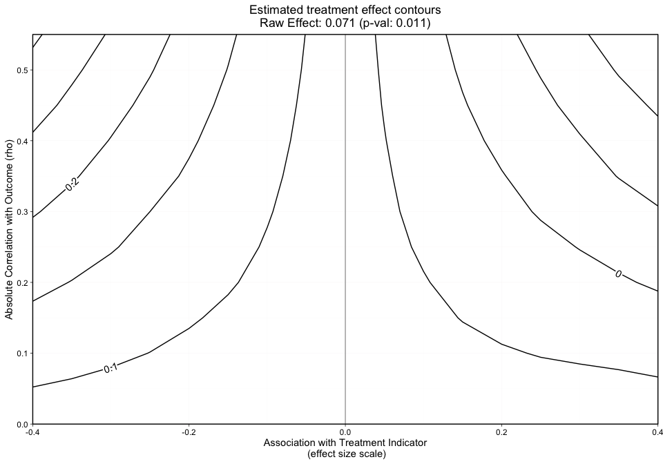
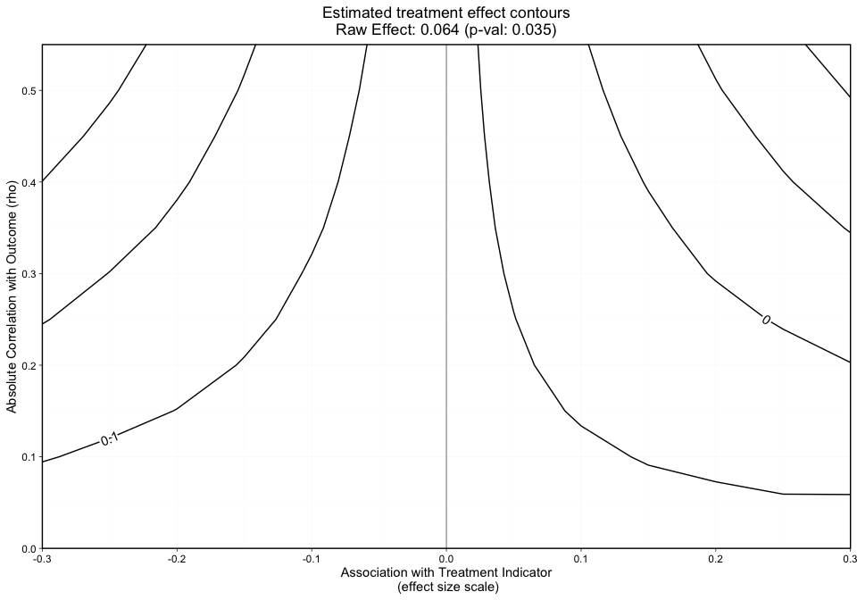
The first graphic (Figure 1) plots the treatment effect contours without covariate labels. This graphic can be produced by specifying print_graphic to “1”. If the user specifies the parameter col as "color", the contours will overlay a colored heat map.
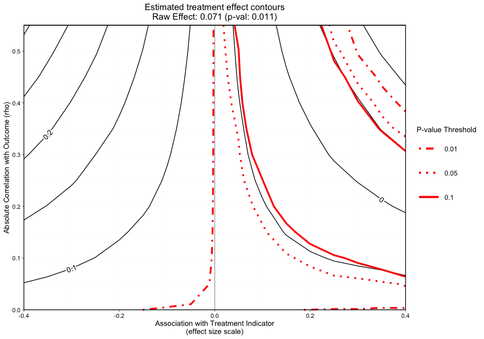
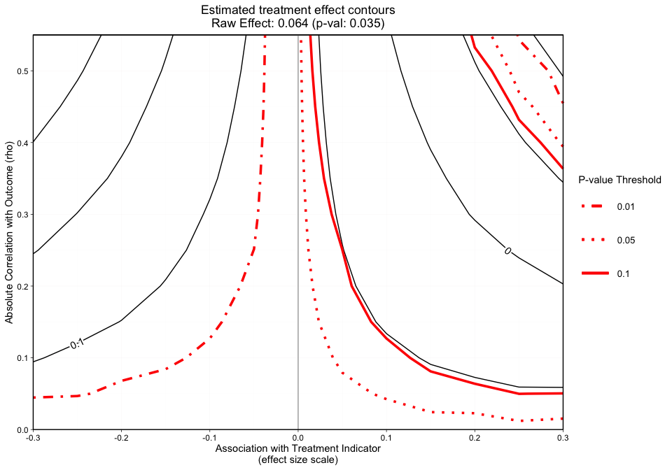
The second graphic (Figure 2) plots the treatment effect contours in black and the p-value contours in red. The p-value contours can be specified with p_contours. The default values are 0.01, 0.05, and 0.1.
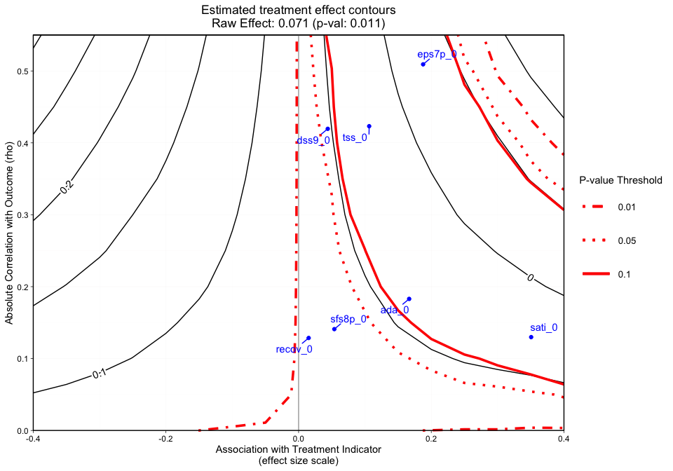
The third graphic (Figure 3) plots the treatment effect contours with the p-value contour overlaid and covariate labels (i.e. the column names submitted to plot_covariates) plotted by their raw rho and effect size.
The following code snippet will produce Figure 1.

The grid, as shown by the x-axis and y-axis in Figure 1 presents the effect size and rho, respectively.
The y-axis in Figure 1 represents the unobserved confounder’s absolute correlation with the outcome and the x-axis is the association between the unobserved confounder and the treatment indicator on an effect size scale. The black lines represent treatment effect contours that run along the grid. The PS weighted treatment effect of Treatment A versus Treatment B equals 0.071 and is significant with a p-value equal to 0.011. However, looking at this graphic alone will not give us an idea of how sensitive statistical significance is.
#> [1] "NOTE: Covariates with absolute correlation with
outcome greater than 0.4: eps7p_0 (Actual: 0.509), tss_0
(Actual: 0.423), dss9_0 (Actual: 0.420)"
Figure 2 is a different variation of Figure 1, but now adds p-value contours. This graphic will allow the user to see what treatment effect will switch the significance level at critical p-values (e.g., 0.05). This graphic will now give the user an idea of how sensitive both the treatment effect estimate and the statistical significance are. The analyst can specify what red p-value thresholds they want plotted with the p_contours argument.
#> [1] "NOTE: Covariates with absolute correlation with
outcome greater than 0.4: eps7p_0 (Actual: 0.509), tss_0
(Actual: 0.423), dss9_0 (Actual: 0.420)"
Figure 3 adds a final dimension (observed covariate labels) to Figure 2. Similar to Figures 1 and 2, plotted at the top of the figure margin is the ps weighted treatment effect (0.071) and associated p-value of 0.011. The solid black contours represent the treatment effect contour lines and the red lines (sometimes dashed) represent the p-value thresholds. The key on the right side of the graphic shows where various p-value cutoff lines are, including p = 0.05. The blue points on the plot represent the observed covariate correlations with the outcome (y-axis) and effect size associations with the treatment indicator (x-axis). For instance, ada_0 and the outcome have approximately a 0.18 absolute correlation with the emotional problem scale at three months and an absolute association of approximately 0.17 effect size difference between the two treatment groups (magnitude of its relationship with the treatment indicator). In this case, if an unobserved confounder had a relationship with the outcome (eps7p_3) and the treatment indicator (treat) that was equivalent to ada_0, tss_0, eps7p_0, sati_0, or dss9_0, then the researcher would conclude that their results would likely be sensitive to an unobserved confounder at a p-value threshold of 0.05. All of these observed relationships are sensitive at the 0.10 p-value threshold other than dss9_0. If the blue points all existed in contours greater than the 0.05 p-value contour, then unobserved confounders with similar associations would retain the significant effect and allow the user to conclude that the results are reasonably robust. Overall, the graphic above showcases an example where findings could be highly sensitive to the effects of an unobserved confounder.
Note: When the outcome model shows a significant effect for all observed covariates, regardless treatment effect direction, we force the sign of the magnitude to go with the direction of the significant effect. The blue points are meant to give the analyst an idea of possible associations (using observed covariates as an indicator) that would change the interpretation of their results.
These results were produced with 50 simulations (n_reps) of the unobserved confounder. If the contours are not smooth or the user wants to add simulations, they can call add_reps and specify the number (more_reps) of additional simulations. Once this is completed, a user can recreate the plots. Example code to add repetitions:
# If you want to add repetitions, run the following line.
# ovtool_results_twang = add_reps(OVtool_results = ovtool_results_twang,
#                                 model_results = results,
#                                 more_reps = 30)
#
# Recreate Graphic
# plot.ov(ovtool_results_twang, print_graphic = "1", col = "bw")Finally, we can interpret this graphic by running the summary command on the ov object:
#>   running simulation [===>-----------]  29% completed in  3s  running simulation [=====>---------]  43% completed in  5s  running simulation [========>------]  57% completed in  8s  running simulation [==========>----]  71% completed in 10s  running simulation [============>--]  86% completed in 13s  running simulation [===============] 100% completed in 15s

#> [1] "Recommendation for reporting the sensitivity
analyses"
#> [1] "The sign of the estimated effect is expected to
remain consistent when simulated unobserved confounders
have the same strength of associations with the treatment
indicator and outcome that are seen in 6 of the 7 observed
confounders. In the most extreme observed case in which the
sign changes, the estimated treatment effect shifts from
0.071 to -0.025. The sign of the estimate would not be
expected to be preserved for unobserved confounders that
have the same strength of association with the treatment
indicator and outcome as eps7p_0."
#> [1] "Statistical significance at the 0.05 level is
expected to be robust to unobserved confounders with
strengths of associations with the treatment indicator and
outcome that are seen in 2 of the 7 observed confounders.
In the most extreme observed case, the p-value would be
expected to increase from 0.011 to 0.372. Significance at
the 0.05 level would not be expected to be preserved for
unobserved confounders that have the same strength of
association with the treatment indicator and outcome as
eps7p_0, sati_0, ada_0, tss_0, dss9_0."
The OVtool gives a recommendation on how to report findings regarding the direction of the treatment effect and statistical significance. An analyst could take the results produced by summary.ov() and adapt the desciption to be included a manuscript. The tool produces these results by iterating through each observed confounder the user specified in the plot_covariates argument to ov_sim and runs the simulation for those exact effect size and rho combinations to produce the treatment effect and p-value. It then determines which observed relationships would produce a treatment effect that changes direction and p-value that crosses over the 0.05 threshold when a significant raw effect is observed.
In the next section, we will show how our method works with the average treatment effect on the treated (ATT) using a continuous outcome.
Perhaps the user is interested in the average treatment effect on the treated. The tool operates very similarly in the ATT setting. We will briefly show the steps needed to run the ATT version of the tool for continuous treatments below. Largely the only difference between ATE and ATT is the user must specify the correct estimand when (1) generating their weights and (2) running their outcome model.
## Create formula - here we use same formula as in the ATE case.
my_formula = as.formula(treat ~ eps7p_0 + sfs8p_0 + sati_0 + ada_0 + recov_0 +
                          tss_0 + dss9_0)

# Propensity score weights:
ps.twang_att <- twang::ps(my_formula, data = sud, estimand = 'ATT',
                          booster = "gbm", stop.method = "ks.max",
                          verbose=F, ks.exact = T)
twang::bal.table(ps.twang_att)
#> $unw
#> tx.mn tx.sd ct.mn ct.sd std.eff.sz stat p ks ks.pval
#> eps7p_0 0.256 0.196 0.219 0.192 0.185 5.937 0.000 0.103 0.000
#> sfs8p_0 11.253 13.134 10.571 12.162 0.052 1.703 0.089 0.045 0.032
#> sati_0 8.233 22.128 2.145 10.658 0.275 11.088 0.000 0.121 0.000
#> ada_0 48.748 33.400 54.236 32.454 -0.164 -5.271 0.000 0.081 0.000
#> recov_0 0.246 0.431 0.240 0.427 0.015 0.479 0.632 0.006 1.000
#> tss_0 2.277 3.525 1.924 3.115 0.100 3.365 0.001 0.043 0.050
#> dss9_0 2.750 2.604 2.638 2.492 0.043 1.390 0.165 0.023 0.666
#>
#> $ks.max.ATT
#> tx.mn tx.sd ct.mn ct.sd std.eff.sz stat p ks ks.pval
#> eps7p_0 0.256 0.196 0.249 0.193 0.034 1.023 0.306 0.025 0.643
#> sfs8p_0 11.253 13.134 10.935 12.623 0.024 0.725 0.469 0.020 0.881
#> sati_0 8.233 22.128 6.399 19.437 0.083 1.840 0.066 0.036 0.207
#> ada_0 48.748 33.400 50.324 33.268 -0.047 -1.365 0.172 0.028 0.489
#> recov_0 0.246 0.431 0.234 0.424 0.027 0.810 0.418 0.012 1.000
#> tss_0 2.277 3.525 2.226 3.440 0.015 0.399 0.690 0.016 0.976
#> dss9_0 2.750 2.604 2.790 2.582 -0.016 -0.446 0.655 0.014 0.992Notice that the only difference here is we use estimand = ATT to estimate the propensity score weights using TWANG. We observe reasonable balance; all of our standardized effect size differences are less than 0.1. As mentioned in the ATE example, refer to Ridgeway et al. for further information on balance diagnostics.
The following code snippet displays how a user would insert a ps object produced by twang into outcome_model and specify the appropriate stopping method to extract the propensity score weights as opposed to utilizing the weights argument. Other than this, the only difference in the call to outcome_model from the ATE example is specifying the correct estimand.
results_att = outcome_model(ps_object = ps.twang_att,
                            stop.method = "ks.max",
                            data = sud,
                            weights = NULL,
                            treatment = "treat",
                            outcome = "eps7p_3_std",
                            model_covariates = c("eps7p_0", "sfs8p_0",
                                                 "sati_0", "ada_0",
                                                 "recov_0", "tss_0",
                                                 "mhtrt_0", "dss9_0"),
                            estimand = "ATT")
summary(results_att$mod_results)
#>
#> Call:
#> svyglm(formula = formula, design = design_u)
#>
#> Survey design:
#> design_u <- survey::svydesign(ids=~1, weights=~w_orig, data=data)
#>
#> Coefficients:
#> Estimate Std. Error t value Pr(>|t|)
#> (Intercept) 0.3492268 0.0669257 5.218 1.90e-07 ***
#> treat 0.0641723 0.0304310 2.109 0.0350 *
#> eps7p_0 1.6430733 0.1242182 13.227 < 2e-16 ***
#> sfs8p_0 0.0026741 0.0021297 1.256 0.2093
#> sati_0 0.0020878 0.0012827 1.628 0.1037
#> ada_0 0.0002505 0.0007861 0.319 0.7500
#> recov_0 -0.0788224 0.0336288 -2.344 0.0191 *
#> tss_0 0.0344397 0.0074878 4.599 4.37e-06 ***
#> mhtrt_0 0.2468881 0.0370127 6.670 2.90e-11 ***
#> dss9_0 0.0481264 0.0081534 5.903 3.88e-09 ***
#> ---
#> Signif. codes: 0 '***' 0.001 '**' 0.01 '*' 0.05 '.' 0.1 ' ' 1
#>
#> (Dispersion parameter for gaussian family taken to be 0.7229591)
#>
#> Number of Fisher Scoring iterations: 2Under the ATT setting, our treatment effect is 0.064 with a p-value of 0.035.
We now want to understand how sensitive our result is to unobserved confounders. Below we will run the ov_sim function; we notice that in our call to ov_sim the parameters remain the same as in our ATE example. The estimand parameter is stored in results_att and carried forward throughout the remainder of the analysis.
ovtool_results_twang_att = ov_sim(model_results=results_att,
                                  plot_covariates=c("eps7p_0", "sfs8p_0",
                                                    "sati_0", "ada_0",
                                                    "recov_0", "tss_0",
                                                    "dss9_0"),
                                  es_grid = NULL,
                                  rho_grid = seq(0, 0.40, by = 0.05),
                                  n_reps = 50,
progress = TRUE)Occasionally the specified number of repetitions (default is n_reps = 50) is not sufficient. Evidence that n_reps is not sufficient are contours that don’t appear smooth. The number of repetitions needed can vary based on sample size, the distribution of the outcome, and the specified estimand. Once we observe our graphical results, if the contours do not look smooth, we recommend calling the add_reps function and specifying more_reps to the number of additional simulations of the unobserved confounder you desire.
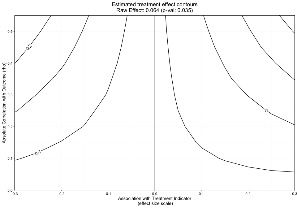
The contours shown in Figure 4 are relatively smooth but for sake of example we show how a user would specify 10 additional repetitions. The user can specify more_reps to any number they choose in the following function call, add_reps().
# If you want to add repetitions, run the following line.
ovtool_results_twang_att = add_reps(OVtool_results = ovtool_results_twang_att,
                                    model_results = results_att,
                                    more_reps = 10)
Once the number of repetitions is finalized, the user can visualize the results through the same three function calls as described in the ATE section above.
To review, the graphics visualize (1) treatment effect contours, (2) treatment effect contours in black and p-value contours in red, and (3) treatment effect and p-value contours with covariate labels added, respectively.
#> [1] "NOTE: Covariates with absolute correlation with
outcome greater than 0.3: eps7p_0 (Actual: 0.509), tss_0
(Actual: 0.423), dss9_0 (Actual: 0.420)"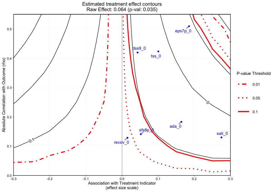
#> [1] "NOTE: Covariates with absolute correlation with
outcome greater than 0.3: eps7p_0 (Actual: 0.509), tss_0
(Actual: 0.423), dss9_0 (Actual: 0.420)"Finally, we will run the summary.ov function to receive the tool’s recommendations.
#>   running simulation [===>-----------]  29% completed in  1s  running simulation [=====>---------]  43% completed in  1s  running simulation [========>------]  57% completed in  2s  running simulation [==========>----]  71% completed in  3s  running simulation [============>--]  86% completed in  4s  running simulation [===============] 100% completed in  4s

#> [1] "Recommendation for reporting the sensitivity
analyses"
#> [1] "The sign of the estimated effect is expected to
remain consistent when simulated unobserved confounders
have the same strength of associations with the treatment
indicator and outcome that are seen in 6 of the 7 observed
confounders. In the most extreme observed case in which the
sign changes, the estimated treatment effect shifts from
0.064 to -0.04. The sign of the estimate would not be
expected to be preserved for unobserved confounders that
have the same strength of association with the treatment
indicator and outcome as eps7p_0."
#> [1] "Statistical significance at the 0.05 level is
expected to be robust to unobserved confounders with
strengths of associations with the treatment indicator and
outcome that are seen in 1 of the 7 observed confounders.
In the most extreme observed case, the p-value would be
expected to increase from 0.035 to 0.583. Significance at
the 0.05 level would not be expected to be preserved for
unobserved confounders that have the same strength of
association with the treatment indicator and outcome as
eps7p_0, sfs8p_0, sati_0, ada_0, tss_0, dss9_0."
The text produced states that the sign of the estimated effect is expected to remain consistent when simulated unobserved confounders have the same strength of associations with the treatment indicator and outcome that are seen in six of the seven observed confounders. On the other hand, statistical significance at the 0.05 alpha level is robust to unobserved confounders with strengths of associations with treatment indicator and outcome that are seen in only one of our observed covariates.
In observational studies, understanding the sensitivity of reported results to unobserved confounders is a key step when interpreting the strength of evidence. This package aims to provide user-friendly tools to assess the sensitivity of research findings to omitted variables when estimating causal effects using PS weighting.
This tutorial and the development of the OVtool R package were supported by funding from grant 1R01DA034065 from the National Institute on Drug Abuse. The overarching goal of the grant is to develop statistical methods and tools that will provide addiction health services researchers and others with the tools and training they need to study the effectiveness of treatments using observational data. The work is an extension of the Toolkit for Weighting and Analysis of Nonequivalent Groups, or TWANG, which contains a set of functions to support causal modeling of observational data through the estimation and evaluation of propensity score weights. The TWANG package was first developed in 2004 by RAND researchers for the R statistical computing language and environment and has since been expanded to include tools for SAS, Stata, and Shiny. For more information about TWANG and other causal tools being developed, see www.rand.org/statistics/twang.
RAND Social and Economic Well-Being is a division of the RAND Corporation that seeks to actively improve the health and social and economic well-being of populations and communities throughout the world. This research was conducted in the Social and Behavioral Policy Program within RAND Social and Economic Well-Being. The program focuses on such topics as risk factors and prevention programs, social safety net programs and other social supports, poverty, aging, disability, child and youth health and well-being, and quality of life, as well as other policy concerns that are influenced by social and behavioral actions and systems that affect well-being. For more information, email sbp@rand.org.
We would like to acknowledge the Center for Substance Abuse Treatment (CSAT), Substance Abuse and Mental Health Services Administration (SAMHSA). The authors thank these agencies, grantees, and their participants for agreeing to share their data to support creation of the synthetic dataset used in this analysis. This tutorial uses a synthetic dataset of youth receiving two unidentified treatments from the GAIN; running on the true dataset will produce different results.
We also would like to thank our beta testers: Irineo Cabreros, Marika Booth, Andreas Markoulidakis, Brooke Hunter, and Yajna Chakraborti. Their comments, feedback, and suggestions were invaluable throughout the development of this tool.
Burgette, L., Griffin, B. A., Pane, J. D., and McCaffrey, D. M. (2021). Got a feeling something is missing? Assessing Sensitivity to Omitted Variables in Substance Use Treatment. arXiv.
Cohen, J. (1988). Statistical Power Analysis for the Behavioral Sciences (2nd ed.). Hillsdale, NJ: Lawrence Erlbaum Associates, Publishers.
Dennis, M. L., Titus, J. C., White, M. K., Unsicker, J. I., & Hodgkins, D. (2003). Global appraisal of individual needs: Administration guide for the GAIN and related measures. Bloomington, IL: Chestnut Health Systems.
Griffin, B.A., Ayer, L., Pane, J., Vegetabile, B.G., Burgette, L.F., McCaffrey, D.M., Coffman, D.L., Cefalu, M., Funk, R., Godley, M. Expanding outcomes when considering the relative effectiveness of two evidence-based outpatient treatment programs for adolescents. 2020. Journal of Substance Abuse Treatment, 118, 108075. PMCID: PMC519172
Lumley, T (2020). “survey: analysis of complex survey samples.” R package version 4.0.
McCaffrey, D. F., Ridgeway, G., and Morral, A. R. (2004). Propensity score estimation with boosted regression for evaluating causal effects in observational studies. Psychological methods 9, 403.
Nowok B, Raab GM, Dibben C (2016). “synthpop: Bespoke Creation of Synthetic Data in R.” Journal of Statistical Software, 74(11), 1–26. doi: 10.18637/jss.v074.i11.
Ridgeway, G., McCaffrey, D., Morral, A., Cefalu, M., Burgette, L., and Griffin, B. A. (2021). Toolkit for Weighting and Analysis of Nonequivalent Groups: A tutorial for the twang package. Santa Monica, CA: RAND Corporation.