


true
Markov Affinity-based Graph Imputation of Cells (MAGIC) is an algorithm for denoising and imputation of single cells applied to single-cell RNA sequencing data, as described in Van Dijk D et al. (2018), Recovering Gene Interactions from Single-Cell Data Using Data Diffusion, Cell https://www.cell.com/cell/abstract/S0092-8674(18)30724-4.
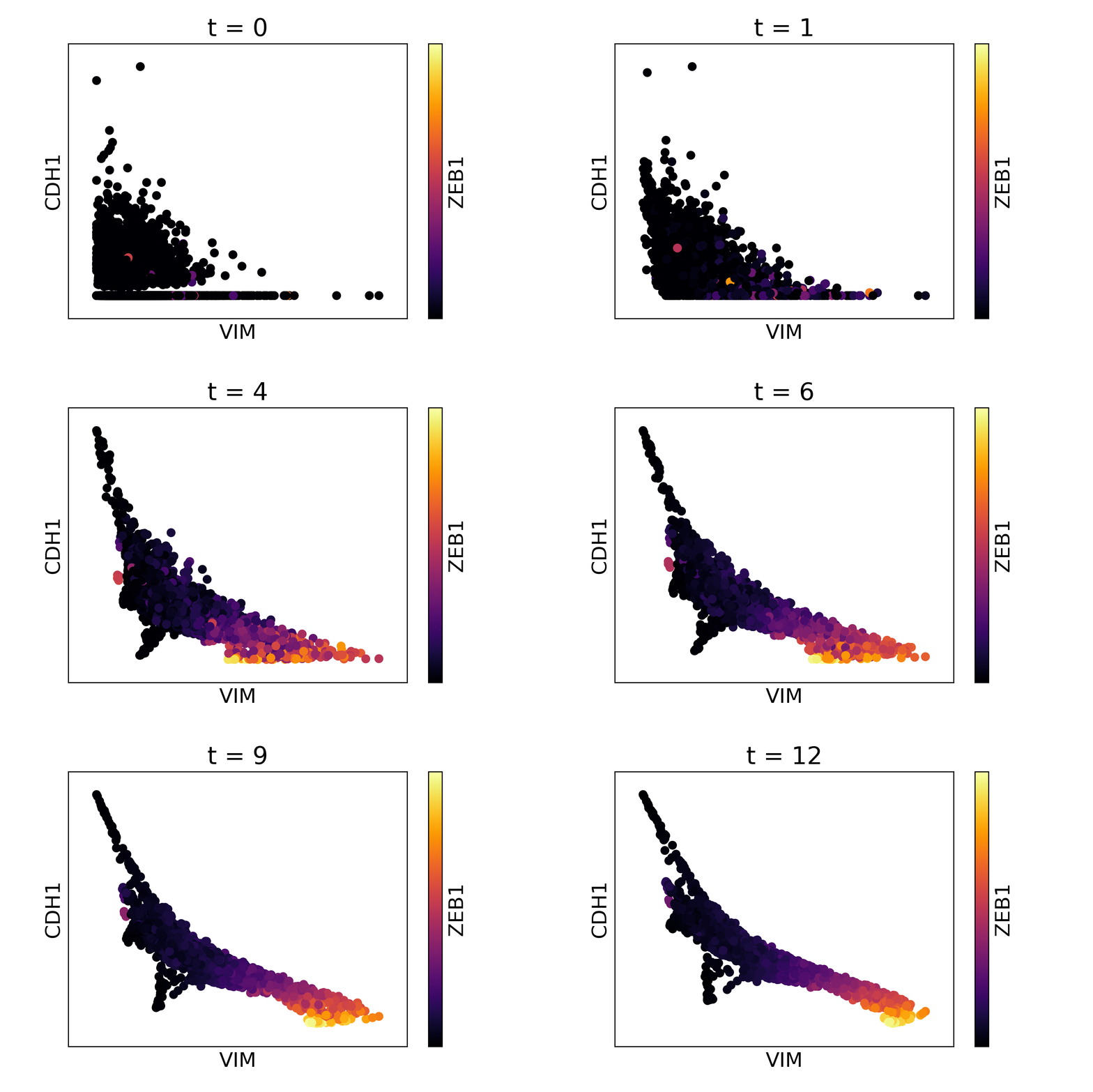
Magic reveals the interaction between Vimentin (VIM), Cadherin-1 (CDH1), and Zinc finger E-box-binding homeobox 1 (ZEB1, encoded by colors).
inst/examples:
To use MAGIC, you will need to install both the R and Python packages.
If python or pip are not installed, you will need to install them. We recommend Miniconda3 to install Python and pip together, or otherwise you can install pip from https://pip.pypa.io/en/stable/installing/.
In R, run this command to install MAGIC and all dependencies:
In a terminal, run the following command to install the Python repository.
To install the very latest version of MAGIC, you can install from GitHub with the following commands run in a terminal.
git clone https://github.com/KrishnaswamyLab/MAGIC
cd MAGIC/python
python setup.py install --user
cd ../Rmagic
R CMD INSTALL .If you have loaded a data matrix data in R (cells on rows, genes on columns) you can run PHATE as follows:
We’ll install a couple more tools for this tutorial.
if (!require(viridis)) install.packages("viridis")
if (!require(ggplot2)) install.packages("ggplot2")
if (!require(phateR)) install.packages("phateR")
If you have never used PHATE, you should also install PHATE from the command line as follows:
We load the Rmagic package and a few others for convenience functions.
library(Rmagic)
#> Loading required package: Matrix
library(ggplot2)
#> Warning: package 'ggplot2' was built under R version 3.5.3
library(viridis)
#> Loading required package: viridisLite
library(phateR)
#>
#> Attaching package: 'phateR'
#> The following object is masked from 'package:Rmagic':
#>
#> library.size.normalizeThe example data is located in the MAGIC R package.
# load data
data(magic_testdata)
magic_testdata[1:5,1:10]
#>       A1BG-AS1     AAMDC      AAMP AARSD1 ABCA12 ABCG2    ABHD13
#> 6564 0.0000000 0.0000000 0.0000000      0      0     0 0.0000000
#> 3835 0.0000000 0.8714711 0.0000000      0      0     0 0.8714711
#> 6318 0.7739207 0.0000000 0.7739207      0      0     0 0.0000000
#> 3284 0.0000000 0.0000000 0.0000000      0      0     0 0.0000000
#> 1171 0.0000000 0.0000000 0.0000000      0      0     0 0.0000000
#>      AC007773.2 AC011998.4 AC013470.6
#> 6564          0          0          0
#> 3835          0          0          0
#> 6318          0          0          0
#> 3284          0          0          0
#> 1171          0          0          0
Running MAGIC is as simple as running the magic function.
We can plot the data before and after MAGIC to visualize the results.
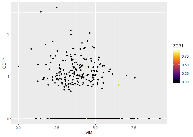
The data suffers from dropout to the point that we cannot infer anything about the gene-gene relationships.
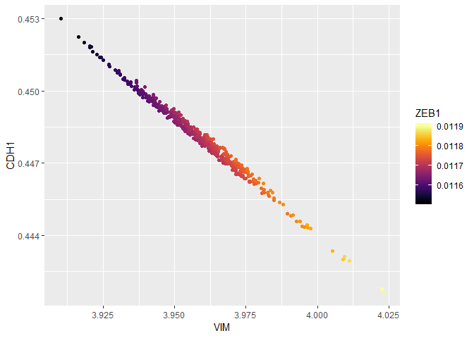
As you can see, the gene-gene relationships are much clearer after MAGIC.
The data is sometimes a little too smooth - we can decrease t from the automatic value to reduce the amount of diffusion. We pass the original result to the argument init to avoid recomputing intermediate steps.
data_MAGIC <- magic(magic_testdata, genes=c("VIM", "CDH1", "ZEB1"), t=6, init=data_MAGIC)
ggplot(data_MAGIC) +
  geom_point(aes(VIM, CDH1, colour=ZEB1)) +
  scale_colour_viridis(option="B")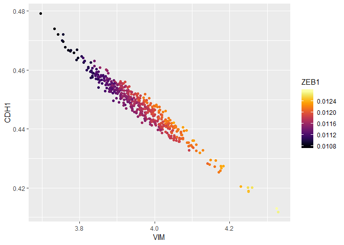
We can look at the entire smoothed matrix with genes='all_genes', passing the original result to the argument init to avoid recomputing intermediate steps. Note that this matrix may be large and could take up a lot of memory.
data_MAGIC <- magic(magic_testdata, genes="all_genes", t=6, init=data_MAGIC)
as.data.frame(data_MAGIC)[1:5, 1:10]
#>        A1BG-AS1      AAMDC      AAMP     AARSD1     ABCA12      ABCG2
#> 6564 0.02565716 0.06303703 0.1726791 0.01559474 0.03114244 0.01423031
#> 3835 0.02535551 0.06286382 0.1678011 0.01547390 0.03017628 0.01428737
#> 6318 0.02619089 0.06298015 0.1744098 0.01514747 0.03145176 0.01477152
#> 3284 0.02517645 0.06254417 0.1684572 0.01559623 0.03015758 0.01414733
#> 1171 0.02651602 0.06289360 0.1729842 0.01514780 0.03162480 0.01480426
#>          ABHD13  AC007773.2  AC011998.4  AC013470.6
#> 6564 0.07100262 0.001129400 0.001880153 0.003215547
#> 3835 0.06989726 0.001086716 0.001847604 0.002833342
#> 6318 0.07165035 0.001203505 0.002044504 0.003550067
#> 3284 0.07066602 0.001039065 0.001723499 0.002822357
#> 1171 0.07094679 0.001236082 0.002133401 0.003450875We can visualize the results of MAGIC on PCA as follows.
data_MAGIC_PCA <- as.data.frame(prcomp(data_MAGIC)$x)
ggplot(data_MAGIC_PCA) +
  geom_point(aes(x=PC1, y=PC2, color=data_MAGIC$result$VIM)) +
  scale_color_viridis(option="B") +
  labs(color="VIM")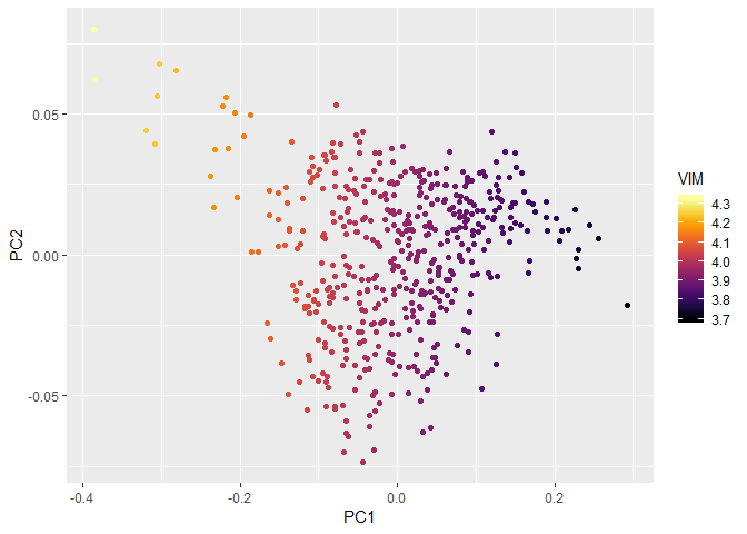
We can visualize the results of MAGIC on PHATE as follows. We set t and k manually, because this toy dataset is really too small to make sense with PHATE; however, the default values work well for single-cell genomic data.
data_PHATE <- phate(magic_testdata, k=3, t=15)
#> Argument k is deprecated. Using knn instead.
ggplot(data_PHATE) +
  geom_point(aes(x=PHATE1, y=PHATE2, color=data_MAGIC$result$VIM)) +
  scale_color_viridis(option="B") +
  labs(color="VIM")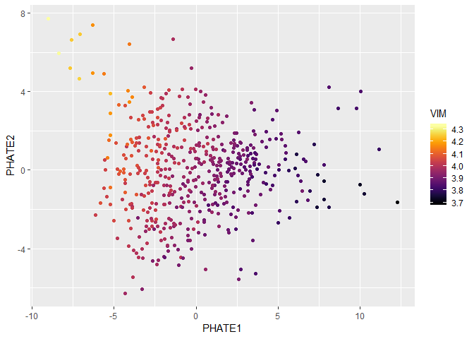
To be consistent with common functions such as PCA (stats::prcomp) and t-SNE (Rtsne::Rtsne), we require that cells (observations) be rows and genes (features) be columns of your input data.
Check your reticulate::py_discover_config("magic") and compare it to the version of Python in which you installed PHATE (run which python and which pip in a terminal.) Chances are reticulate can’t find the right version of Python; you can fix this by adding the following line to your ~/.Renviron:
PATH=/path/to/my/python
You can read more about Renviron at https://cran.r-project.org/package=startup/vignettes/startup-intro.html.
Please let us know of any issues at the GitHub repository. If you have any questions or require assistance using MAGIC, please read the documentation by running help(Rmagic::magic) or contact us at https://krishnaswamylab.org/get-help.