README

Robust Bayesian Meta-Analysis (RoBMA)

This package estimates an ensemble of meta-analytic models (assuming either the presence or absence of effect, heterogeneity, and publication bias) and uses Bayesian model averaging to combine them. The ensemble uses Bayes factors to test for the presence of absence of the individual components (e.g., effect vs. no effect) and model-averages parameter estimates based on posterior model probabilities. The user can define a wide range of non-informative or informative priors for the effect size, heterogeneity, and publication bias components (including selection, PET, and PEESE style models). The package provides convenient functions for summary, visualizations, and fit diagnostics.

See our new pre-print Bartoš et al. (2021) (https://doi.org/10.31234/osf.io/kvsp7) for the description of the newest version, RoBMA-PSMA, or our previous paper introducing the method Maier et al. (in press) (https://doi.org/10.31234/osf.io/u4cns). The previous version of the methods is also implemented within the the user-friendly graphical user interface of JASP (JASP Team, 2020) and accompanied by a tutorial paper with more examples (Bartoš et al., in press) (https://doi.org/10.31234/osf.io/75bqn).

We also prepared multiple vignettes that illustrate functionality of the package:

• Reproducing Bayesian model-averaged meta-analysis (BMA)
• Fitting custom meta-analytic ensembles
• Informed Bayesian model-averaged meta-analysis in medicine

Updates

The package was updated to version 2.0 to provides Bayesian model-averaging across selection models and PET-PEESE (as described in Bartoš et al. (2021) at https://doi.org/10.31234/osf.io/kvsp7).

Backwards Compatibility

Please note that the RoBMA 2.0 is not backwards compatible with the previous versions of RoBMA. Use

remotes::install_version("RoBMA", version = "1.2.1")

to install the previous version if needed. (Or use the source packages archived with at OSF repositories associated with the corresponding projects.)

News

The 2.0 version brings several updates to the package:

• naming of the arguments specifying prior distributions for the different parameters/components of the models changed (priors_mu -> priors_effect, priors_tau -> priors_heterogeneity, and priors_omega -> priors_bias),
• prior distributions for specifying weight functions now use a dedicated function (prior(distribution = "two.sided", parameters = ...) -> prior_weightfunction(distribution = "two.sided", parameters = ...)),
• new dedicated function for specifying no publication bias adjustment component / no heterogeneity component (prior_none()),
• new dedicated functions for specifying models with the PET and PEESE publication bias adjustments (prior_PET(distribution = "Cauchy", parameters = ...) and prior_PEESE(distribution = "Cauchy", parameters = ...)),
• new default prior distribution specification for the publication bias adjustment part of the models (corresponding to the RoBMA-PSMA model from Bartoš et al. (2021)),
• new model_type argument allowing to specify different “pre-canned” models ("PSMA" = RoBMA-PSMA, "PP" = RoBMA-PP, "2w" = corresponding to Maier et al. (in press)),
• combine_data function allows combination of different effect sizes / variability measures into a common effect size measure (also used from within the RoBMA function)
• better and improved automatic fitting procedure now enabled by default (can be turned of with autofit = FALSE)
• prior distributions can be specified on the different scale than the supplied effect sizes (the package fits the model on Fisher’s z scale and back transforms the results back to the scale that was used for prior distributions specification, Cohen’s d by default, but both of them can be overwritten with the prior_scale and transformation arguments),
• new prior distributions, e.g., beta or fixed weight functions,
• and plenty of small changes to the arguments, output, and etc…

Installation

The package requires JAGS 4.3.1 to be installed. The release version can be installed from CRAN:

install.packages("RoBMA")

and the development version of the package can be installed from GitHub:

devtools::install_github("fbartos/RoBMA")

Example

To illustrate the functionality of the package, we fit the RoBMA-PSMA model from the example in Bartoš et al. (2021) to adjust for publication bias in the infamous Bem (2011) “Feeling the future” pre-cognition study. The RoBMA-PSMA model combines six selection models and PET-PEESE to adjust for publication bias. As in the pre-print, we analyze the data as described by Bem et al. (2011) in his reply to methodological critiques.

First, we load the package and the data set included in the package.

library(RoBMA)
#> Loading required namespace: runjags
#> Loading required namespace: mvtnorm
#> module RoBMA loaded

data("Bem2011", package = "RoBMA")
Bem2011
#>      d         se                                        study
#> 1 0.25 0.10155048                  Detection of Erotic Stimuli
#> 2 0.20 0.08246211                Avoidance of Negative Stimuli
#> 3 0.26 0.10323629                        Retroactive Priming I
#> 4 0.23 0.10182427                       Retroactive Priming II
#> 5 0.22 0.10120277  Retroactive Habituation I - Negative trials
#> 6 0.15 0.08210765 Retroactive Habituation II - Negative trials
#> 7 0.09 0.07085372             Retroactive Induction of Boredom
#> 8 0.19 0.10089846                     Facilitation of Recall I
#> 9 0.42 0.14752627                    Facilitation of Recall II

Then, we fit the meta-analytic model ensemble that is composed of 36 models (the new default settings of RoBMA fitting function). These models represent all possible combinations of prior distributions for the following components:

• effect size (the mean parameter )
  • a spike at zero, representing the null hypothesis of the absence of effect
  • a standard normal distribution, representing the alternative hypothesis of the presence of effect
• heterogeneity (the heterogeneity parameter )
  • a spike at zero, representing the null hypothesis of the absence of heterogeneity (i.e., fixed effect meta-analysis)
  • an inverse gamma distribution with shape = 1 and scale = 0.15, based on Erp et al. (2017), representing the alternative hypothesis of the presence of heterogeneity (i.e., random effect meta-analysis)
• publication bias
  • no prior distribution, representing the absence of publication bias
  • eight prior distributions specifying two two-sided weight functions, four one-sided weight functions, and PET and PEESE publication bias adjustment, representing the presence of publication bias

The prior odds of the components are by default set to make all three model categories equally likely a priory (0.5 prior probability of the presence of the effect, 0.5 prior probability of the presence of the heterogeneity, and 0.5 prior probability of the presence of the publication bias). The prior model probability of the publication bias adjustment component is further split equally among the selection models represented by the six weightfunctions and the PET-PEESE models.

fit <- RoBMA(d = Bem2011$d, se = Bem2011$se, study_names = Bem2011$study, seed = 1)

The main summary can be obtained using the summary.RoBMA() function.

The first table shows an overview of the ensemble composition. The number of models, the prior and posterior model probabilities, and inclusion Bayes factor of the ensemble components representing the alternative hypothesis of the presence of the effect, heterogeneity, and publication bias, We can see the data show very weak evidence, barely worth mentioning, against the presence of the effect ( -> ), moderate evidence for the absence of heterogeneity ( -> ), and strong evidence for the presence of publication bias ().

The second table shows model-averaged estimates weighted by the individual models’ posterior probabilities. The mean estimate , 95% CI [-0.041, 0.213], is very close to zero, corresponding to the a priory expected absence of pre-cognition. The heterogeneity estimate has most of its probability mass around zero due to the higher support of models assuming absence of the heterogeneity. The parameters omega, representing the publication weights at each p-value interval are decreasing with increasing p-values, showing the publication bias, as well as the non zero PET and PEESE estimates.

summary(fit)
#> Call:
#> RoBMA(d = Bem2011$d, se = Bem2011$se, study_names = Bem2011$study, 
#>     seed = 1)
#> 
#> Robust Bayesian meta-analysis
#> Components summary:
#>               Models Prior prob. Post. prob. Inclusion BF
#> Effect         18/36       0.500       0.324        0.479
#> Heterogeneity  18/36       0.500       0.125        0.143
#> Bias           32/36       0.500       0.942       16.323
#> 
#> Model-averaged estimates:
#>                    Mean Median  0.025  0.975
#> mu                0.037  0.000 -0.041  0.213
#> tau               0.010  0.000  0.000  0.113
#> omega[0,0.025]    1.000  1.000  1.000  1.000
#> omega[0.025,0.05] 0.935  1.000  0.338  1.000
#> omega[0.05,0.5]   0.780  1.000  0.009  1.000
#> omega[0.5,0.95]   0.768  1.000  0.007  1.000
#> omega[0.95,0.975] 0.786  1.000  0.007  1.000
#> omega[0.975,1]    0.801  1.000  0.007  1.000
#> PET               0.759  0.000  0.000  2.805
#> PEESE             6.183  0.000  0.000 25.463
#> The estimates are summarized on the Cohen's d scale (priors were specified on the Cohen's d scale).
#> (Estimated publication weights omega correspond to one-sided p-values.)

We can visualize the estimated mean and heterogeneity parameters using the plot.RoBMA() function. The arrows in both figures represent the point probability mass at and , corresponding to the null hypotheses of the absence of effect and heterogeneity, both increasing in the posterior model probability from 0.5 to 0.676 and 0.875 respectively.

plot(fit, parameter = "mu", xlim = c(-0.5, 0.5))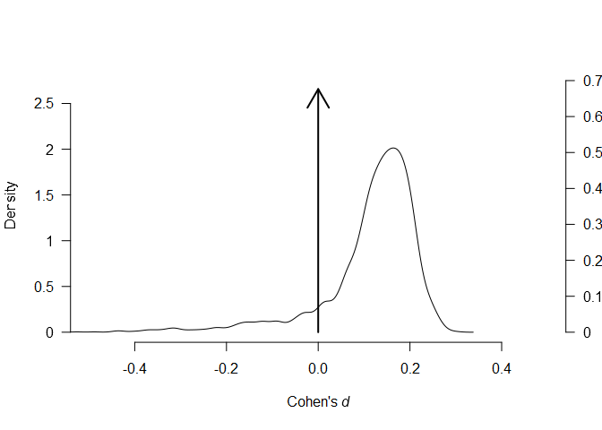

plot(fit, parameter = "tau")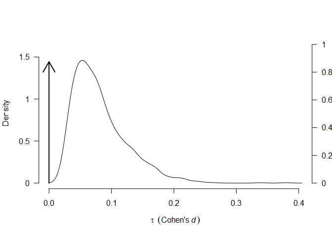

We can further visualize the publication bias adjustments of selection models, visualizing the posterior estimate of the model-averaged weightfunction that shows a sharp decrease in the publication weights of studies with p-values above the “marginal significance” (0.10) level,

plot(fit, parameter = "weightfunction", rescale_x = TRUE)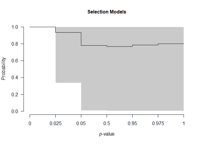

and the PET-PEESE publication bias adjustment, visualizing the individual studies’ standard errors and effect sizes as diamonds and the model-averaged estimate of the regression lines that shows a steady increase of effect sizes with increasing standard errors.

plot(fit, parameter = "PET-PEESE", xlim = c(0, 0.25))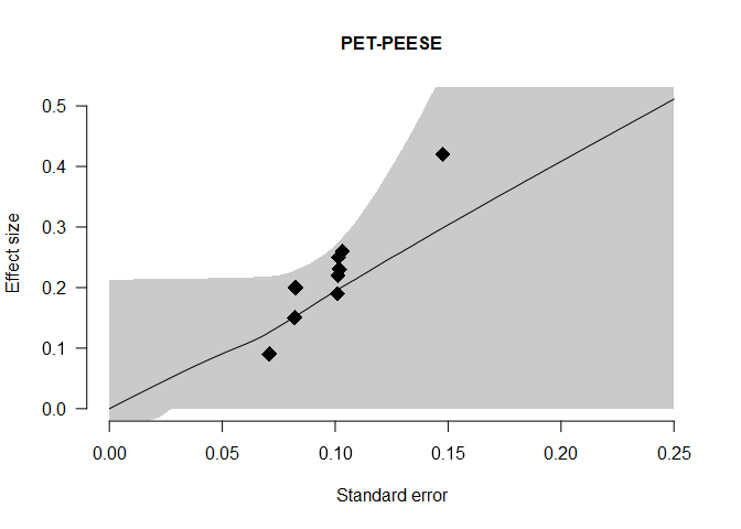

The usual meta-analytic forest plot can be obtained with the forest() function,

forest(fit)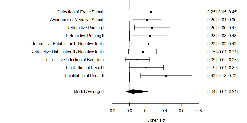

and visualization of the effect size estimates from models assuming presence of the effect can be obtained with the plot_models() function.

plot_models(fit, conditional = TRUE)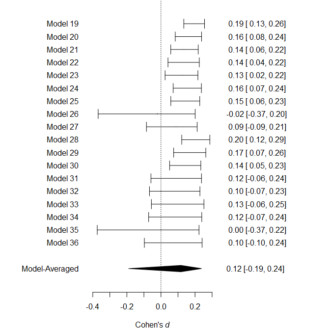

Apart from plotting, the individual model performance can be inspected using the summary.RoBMA() function with argument type = "models" or the overview of the individual model MCMC diagnostics can be obtained by setting type = "diagnostics" (not shown here for the lack of space).

We can also visualize the MCMC diagnostics using the diagnostics function. The function can display the chains type = "chain" / posterior sample densities type = "densities", and averaged auto-correlations type = "autocorrelation". Here, we request the chains trace plot of the parameter of the most complex model by setting show_models = 36 (the model numbers can be obtained from the summary function with type = "models" argument).

diagnostics(fit, parameter = "mu", type = "chains", show_models = 36)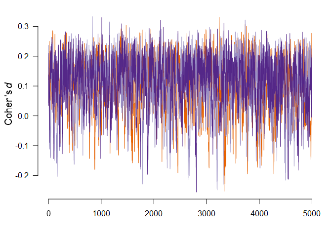

The package allows to fit highly customized models with different prior distribution functions, prior model probabilities, and provides more visualization options. See the documentation to find out more about the specific functions: RoBMA(), priors(), plot.RoBMA(). The main package functionality is also implemented within the Meta Analysis module of JASP 0.14 (JASP Team, 2020) and will be soon updated to accommodate the 2.0 version of the package.

References