This package re-implements measures of ecological diversity from several other software packages, including vegan, scikit-bio, Mothur, and GUniFrac.
You can install abdiv from github with:
Let’s say we’ve surveyed a field and counted the number of plants in each of two sites. We’ve found five species in total, and we’d like to summarize the diversity of the two sampling sites. The diversity within each site is called α-diversity.
Here are the number of plants for each species at site 1 and site 2, represented as vectors.
The two sites have about the same number of total plants, but the distribution of species is much different. More than half the plants in site 1 belong to a single species, whereas the plants in site 2 are almost evenly distributed across three different species. To get started, let’s look at a few ways to quantify the α-diversity for each sample.
Richness measures the total number of species in each sample.
The Shannon index measures both the number of species and the evenness of the relative abundance values. Site 2 has fewer species, but each species has the same relative abundance, so the Shannon index is higher.
Let’s summarize the diversity of site 1 and site 2 using all the functions available in this library. The full set of within-sample diversity functions is available as a character vector in alpha_diversities. The term “α-diversity” means the diversity within a single sample.
library(tidyverse)
tibble(Site = rep(c("Site 1", "Site 2"), each=5), Counts = c(site1, site2)) %>%
  group_by(Site) %>%
  summarize_at(vars(Counts), alpha_diversities) %>%
  pivot_longer(-Site, names_to = "Measure") %>%
  ggplot(aes(x=Measure, y=value, color=Site)) +
  geom_point() +
  scale_color_manual(values=c("#E64B35", "#4DBBD5")) +
  coord_flip() +
  theme_bw()
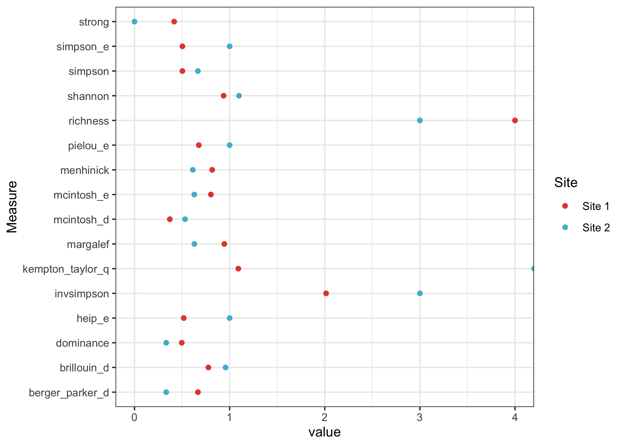
We can see that site 1 is regarded as more diverse by some measures; it has the most species. For other measures, site 2 is regarded as more diverse; it has the most even distribution of species.
In our documentation, you can find more info on each α-diversity function.
Having assessed the diversity within each sample, we can next ask about the number of shared species between sites. If species are shared, how similar is the distribution across species? There are many ways to quantify the between-sample diversity or β-diversity.
You can think about β-diversity as either the similarity or dissimilarity between sites. The functions in abdiv are written in terms of dissimilarity: similar sites will have values close to zero, and highly dissimilar sites will have values close to the maximum. This way of thinking goes along with our intuition about diversity: sites with greater dissimilarity will exhibit increased diversity if we consider both sites together.
Let’s look at some examples. The Jaccard distance counts the fraction of species present in only one site. The answer is 3 out of 5, or 0.6.
The Bray-Curtis dissimilarity adds up the absolute differences between species counts, then divides by the total counts. For our two sites, that’s (2 + 5 + 8 + 8 + 7) / 48, or 0.625.
Again, we’ll use a vector called beta_diversities to compute every dissimilarity measure in the library.
tibble(Measure = beta_diversities) %>%
  group_by(Measure) %>%
  mutate(value = get(Measure)(site1, site2)) %>%
  ggplot(aes(x=Measure, y=value)) +
  geom_point(color="#4DBBD5") +
  scale_y_log10() +
  coord_flip() +
  theme_bw()
The dissimilarities are generally positive, and they have a range of scales. Some dissimilarity measures range from 0 to 1, while others can go up indefinitely.
As before, you can find more info on each β-diversity function in our documentation.
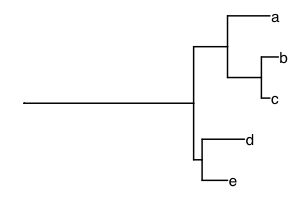
A phylogenetic tree can be incorporated into diversity measures to add information about the evolutionary history of species. One of the first measures in this area was Faith’s phylogenetic diversity. Here, we take an example from Figure 1 in Faith and Richards (PMID 24832524) to show how phylogenetic diversity works. The tree is included as faith_tree:

If all the species are present, the value of Faith’s phylogenetic diversity (PD) is the sum of the branch lengths. Here, we expect the total branch length to be 5 + 4 + 2 + 4 + 1 + 20 + 5 + 1 + 3 = 45, adding from top to bottom.[1]
Here is how you would calculate Faith’s PD:
If species “a” is missing, we expect Faith’s PD to be reduced by 5, the length of the branch leading to species “a”.
The practice of using phylogenetic information in diversity has been especially popular in microbial ecology, where bacteria are surveyed using the 16S rRNA marker gene. In addition to serving as a fingerprint for bacteria, the gene sequence can be used to build a phylogenetic tree.
In this area, the UniFrac distance is widely used to measure β-diversity between bacterial communities. We’ll reproduce an example from the UniFrac paper by Lozupone and Knight (PMID 16332807), which describes the unweighted UniFrac distance. The tree from Figure 1 is available as lozupone_tree.
In the example from Figure 1A, we’ve measured two bacterial communities, where the species detected in each are labeled with circles and squares. The communities have no species in common.
ggtree(lozupone_tree, ladderize = F) %<+%
  lozupone_panel_a +
  geom_tippoint(aes(shape=SampleID), x=2.6, size=3) +
  scale_shape_manual(values = c(1, 15)) +
  scale_x_continuous(limits=c(0, 2.8))
The circle and square communities are all mixed up on the phylogenetic tree. The unweighted UniFrac distance is the fraction of the total branch length where the branch leads to a circle or square, but not both. Here, we would only count the branches leading to the tips of the tree. The length of these branches, added together, is about half the total length for all branches in the tree.
a_circle <- c(1, 0, 1, 1, 0, 1, 0, 0, 1, 0, 0, 1, 0, 1)
a_square <- c(0, 1, 0, 0, 1, 0, 1, 1, 0, 1, 1, 0, 1, 0)
unweighted_unifrac(a_circle, a_square, lozupone_tree)
## [1] 0.5378151
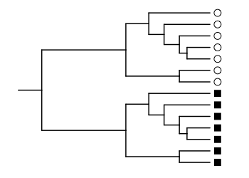
We can increase the UniFrac distance if we rearrange the communities so that all the circles are in the upper part of the tree and all the squares are in the lower part. In the paper, this is shown in Figure 1B.
ggtree(lozupone_tree, ladderize = F) %<+%
  lozupone_panel_b +
  geom_tippoint(aes(shape=SampleID), x=2.6, size=3) +
  scale_shape_manual(values = c(1, 15)) +
  scale_x_continuous(limits=c(0, 2.8))
With this arrangement, the species in each community are phylogenetically very different. Except for the root, each branch of the tree leads uniquely to a species present in square or circle, and never to a species present in both. Therefore, the UniFrac distance is close to 1.
b_circle <- c(1, 1, 1, 1, 1, 1, 1, 0, 0, 0, 0, 0, 0, 0)
b_square <- c(0, 0, 0, 0, 0, 0, 0, 1, 1, 1, 1, 1, 1, 1)
unweighted_unifrac(b_circle, b_square, lozupone_tree)
## [1] 0.9747899Now that we’ve introduced you to the functions in this package, we should probably tell you how to use them in your work. Your data are likely to be in one of two formats: a long-format data frame, or a matrix of counts. We’ll tackle the long format first.
First, we’ll arrange the data from the plant survey example in long format. We’ll also add a third site to help with the demonstration.
site3 <- c(15, 1, 4, 2, 2)
plants <- tibble(
  Site = rep(c("Site 1", "Site 2", "Site 3"), each = 5),
  Species = rep(letters[1:5], times = 3),
  Counts = c(site1, site2, site3)
)
plants
## # A tibble: 15 x 3
##    Site   Species Counts
##    <chr>  <chr>    <dbl>
##  1 Site 1 a            2
##  2 Site 1 b            5
##  3 Site 1 c           16
##  4 Site 1 d            0
##  5 Site 1 e            1
##  6 Site 2 a            0
##  7 Site 2 b            0
##  8 Site 2 c            8
##  9 Site 2 d            8
## 10 Site 2 e            8
## 11 Site 3 a           15
## 12 Site 3 b            1
## 13 Site 3 c            4
## 14 Site 3 d            2
## 15 Site 3 e            2
If we want to compute α-diversity, we can group by Site and create a new column with the answer. The α-diversity functions take the number of counts for each species as an argument.
plants %>%
  group_by(Site) %>%
  summarize(Richness = richness(Counts))
## # A tibble: 3 x 2
##   Site   Richness
##   <chr>     <int>
## 1 Site 1        4
## 2 Site 2        3
## 3 Site 3        5
If you want to cover more than one α-diversity measure, you can use summarize_at().
plants %>%
  group_by(Site) %>%
  summarise_at(vars(Counts), c("shannon", "invsimpson"))
## # A tibble: 3 x 3
##   Site   shannon invsimpson
##   <chr>    <dbl>      <dbl>
## 1 Site 1   0.937       2.01
## 2 Site 2   1.10        3
## 3 Site 3   1.14        2.30
The old school way to compute α-diversity is to arrange your data in a matrix format, with rows representing different sites or “observations”, and columns representing species. This is how you would do it with the vegan package, for example. Here is our data in matrix format:
plants_matrix <- matrix(
  c(site1, site2, site3), nrow=3, byrow=TRUE,
  dimnames = list(c("Site 1", "Site 2", "Site 3"), letters[1:5]))
plants_matrix
##         a b  c d e
## Site 1  2 5 16 0 1
## Site 2  0 0  8 8 8
## Site 3 15 1  4 2 2
In matrix format, we can use the apply() function from base R to get the diversity for each site.
Here is the same example using vegan.
The long format is friendlier to workflows using functions in the tidyverse, but the matrix format has some advantages. The matrix format ensures that every sample has a valid count value for every species considered; the matrix contains values of zeros for species not observed. This quality is not critically important for alpha-diversity measures, but it is important for computing β-diversity.
For β-diversity, we recommend proceeding via the matrix format. If your data is in long format, the usedist package has a function to convert to a numeric matrix.[2]
usedist::pivot_to_numeric_matrix(plants, Site, Species, Counts)
##         a b  c d e
## Site 1  2 5 16 0 1
## Site 2  0 0  8 8 8
## Site 3 15 1  4 2 2
To create a distance matrix between samples, we can employ the dist_make() function from usedist.
usedist::dist_make(plants_matrix, bray_curtis)
##           Site 1    Site 2
## Site 2 0.6250000
## Site 3 0.6666667 0.6666667One practical issue with phylogenetic diversity is to make sure that the order of the species in your vectors matches the order of the tree. If your vector is not named, and you’re sure that the order matches, you can use the phylogenetic diversity functions as above. To take the example from Faith’s phylogenetic diversity, let’s say we had a vector representing 10 counts of species “d” and 12 of species “e”.
If your vector is named, the names will be automatically used to match the vector with the tree. Missing names are filled in with zero counts.
If your vector is not named, or if you’re not totally sure that the order of species in your vector matches the order of species in the tree, you can pass in the species labels for your vector as an additional argument.
This last approach is useful for a tidyverse workflow, where the vectors are not named and the species labels are found in a separate column. Here is an example for data in long format, where the species labels are in the column, “Species”:
plants %>%
  group_by(Site) %>%
  summarize(FaithPD = faith_pd(Counts, faith_tree, Species))
## # A tibble: 3 x 2
##   Site   FaithPD
##   <chr>    <dbl>
## 1 Site 1      40
## 2 Site 2      38
## 3 Site 3      45
The rules are the same for phylogenetic β-diversity functions. The dist_make() function from usedist will pass along additional keyword arguments to the distance function, so you can give the tree and species labels to dist_make(). Here’s an example from the plants matrix.
usedist::dist_make(plants_matrix, unweighted_unifrac, faith_tree)
##           Site 1    Site 2
## Site 2 0.2666667
## Site 3 0.1111111 0.1555556
Now, we’ll re-order the species in the data matrix to see how things work.
species_reorder <- c("d", "e", "a", "b", "c")
plants_matrix_reorder <- plants_matrix[,species_reorder]
plants_matrix_reorder
##        d e  a b  c
## Site 1 0 1  2 5 16
## Site 2 8 8  0 0  8
## Site 3 2 2 15 1  4
The column names of the matrix are automatically added to vectors extracted from the matrix, so we get the same result as before.
usedist::dist_make(plants_matrix_reorder, unweighted_unifrac, faith_tree)
##           Site 1    Site 2
## Site 2 0.2666667
## Site 3 0.1111111 0.1555556
If the column names are missing, first of all, you’re probably in trouble. But if you do have the species labels stored in a separate vector, you can pass them along to the distance function. Let’s remove the column names from our matrix to check this out.
plants_matrix_reorder_nonames <- plants_matrix_reorder
colnames(plants_matrix_reorder_nonames) <- NULL
plants_matrix_reorder_nonames
##        [,1] [,2] [,3] [,4] [,5]
## Site 1    0    1    2    5   16
## Site 2    8    8    0    0    8
## Site 3    2    2   15    1    4
Now, we can pass the species labels to dist_make() and verify that we get the correct answer.
usedist::dist_make(
  plants_matrix_reorder_nonames, unweighted_unifrac, faith_tree,
  species_reorder)
##           Site 1    Site 2
## Site 2 0.2666667
## Site 3 0.1111111 0.1555556Please don’t hesitate to reach out via email or file an issue if you need support when using this library.
The answer here is slightly different than that in the paper. See faith_tree documentation for further explanation.
Full disclosure: usedist and abdiv are authored by the same person.