Functions for the determination of similarity of highly variable dissolution profiles of two drug formulations are provided. Estimation of f1, f2 and bootstrap f2 is implemented. In addition, functions following the model-independent MCR (multivariate confidence region) procedure and the T2-test for equivalence procedure are available.
So far, the package has not yet been submitted to CRAN. The development version is available from GitHub. Installation from this source is easily done by using install_github() function from the devtools package:
Example 1 illustrates how to solve a common problem by aid of the bootstrap f2 procedure proposed by Shah et al. (1998) using a data set containing the dissolution data of one reference batch and one test batch of n = 12 tablets each, i.e. the dissolution profiles of the % drug release observed at 0, 30, 60, 90 and 180 minutes (See Shah et al. (1998), Table 4).
library(disprofas)

# Data frame
str(dip2)
#> 'data.frame':    72 obs. of  8 variables:
#>  $ type  : Factor w/ 2 levels "Reference","Test": 1 1 1 1 1 1 1 1 1 1 ...
#>  $ tablet: Factor w/ 12 levels "1","2","3","4",..: 1 2 3 4 5 6 7 8 9 10 ...
#>  $ batch : Factor w/ 6 levels "b0","b1","b2",..: 1 1 1 1 1 1 1 1 1 1 ...
#>  $ t.0   : int  0 0 0 0 0 0 0 0 0 0 ...
#>  $ t.30  : num  36.1 33 35.7 32.1 36.1 34.1 32.4 39.6 34.5 38 ...
#>  $ t.60  : num  58.6 59.5 62.3 62.3 53.6 63.2 61.3 61.8 58 59.2 ...
#>  $ t.90  : num  80 80.8 83 81.3 72.6 83 80 80.4 76.9 79.3 ...
#>  $ t.180 : num  93.3 95.7 97.1 92.8 88.8 97.4 96.8 98.6 93.3 94 ...

# Perform estimation and print a summary
res1 <- bootstrap_f2(data = dip2[dip2$batch %in% c("b0", "b4"), ],
                         tcol = 5:8, grouping = "batch",
                         R = 200, new_seed = 421, use_EMA = "no")

class(res1)
#> [1] "bootstrap_f2"
summary(res1)
#>
#> STRATIFIED BOOTSTRAP
#>
#>
#> Call:
#> boot(data = data, statistic = get_f2, R = R, strata = data[,
#>     grouping], grouping = grouping, tcol = tcol[ok])
#>
#>
#> Bootstrap Statistics :
#>     original      bias    std. error
#> t1* 50.07187 -0.02553234   0.9488015
#>
#>
#> BOOTSTRAP CONFIDENCE INTERVAL CALCULATIONS
#> Based on 200 bootstrap replicates
#>
#> CALL :
#> boot.ci(boot.out = t_boot, conf = confid, type = "all", L = jack$loo.values)
#>
#> Intervals :
#> Level      Normal              Basic
#> 90%   (48.54, 51.66 )   (48.46, 51.71 )
#>
#> Level     Percentile            BCa
#> 90%   (48.43, 51.68 )   (48.69, 51.99 )
#> Calculations and Intervals on Original Scale
#> Some BCa intervals may be unstable
#>
#>
#> Shah's lower 90% BCa confidence interval:
#>  48.64613

# Prepare graphical representation
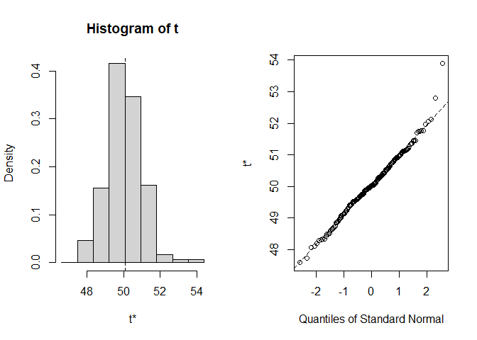
plot(res1)
#>
#> Shah's lower 90% BCa confidence interval:
#>  48.64613
Example 2 illustrates how to solve a common problem by aid of the model-independent non-parametric multivariate confidence region (MCR) procedure proposed by Tsong et al. (1996) using a data set containing the dissolution data of one reference batch and one test batch of n = 6 tablets each, i.e. the dissolution profiles of the % drug release observed at 5, 10, 15, 20, 30, 60, 90 and 120 minutes (see Tsong et al. (1996), Table 1).
library(disprofas)

# Data frame
str(dip3)
#> 'data.frame':    24 obs. of  6 variables:
#>  $ cap  : Factor w/ 12 levels "1","2","3","4",..: 1 2 3 4 5 6 7 8 9 10 ...
#>  $ batch: Factor w/ 2 levels "blue","white": 2 2 2 2 2 2 2 2 2 2 ...
#>  $ type : Factor w/ 2 levels "ref","test": 1 1 1 1 1 1 1 1 1 1 ...
#>  $ x.15 : num  49 15 56 57 6 62 23 11 9 42 ...
#>  $ x.20 : num  86 59 84 87 58 90 71 64 61 81 ...
#>  $ x.25 : num  98 96 96 99 90 97 97 92 88 96 ...

# Perform estimation and print a summary
res2 <- mimcr(data = dip3, tcol = 4:6, grouping = "batch")

class(res2)
#> [1] "mimcr"
summary(res2)
#>
#> Results of Model-Independent Multivariate Confidence Region (MIMCR)
#> approach to assess equivalence of highly variable in-vitro
#> dissolution profiles of two drug product formulations
#>
#> Did the Newton-Raphson search converge? Yes
#>
#> Parameters (general):
#> Significance level:                   0.05
#> Degrees of freedom (1):               3
#> Degrees of freedom (2):               20
#> Mahalanobis distance (MD):            0.2384
#> (F) scaling factor K:                 1.818
#> (MD) scaling factor k:                6
#> Hotelling's T2:                       0.341
#>
#> Parameters specific for Tsong (1996) approach:
#> Maximum tolerable average difference: 10
#> Similarity limit:                     2.248
#> Observed upper limit:                 1.544
#>
#> Parameters specific for Hoffelder (2016) approach:
#> Noncentrality parameter:              30.32
#> Critial F (Hoffelder):                4.899
#> Probability p (Hoffelder):            2.891e-08
#>
#> Conclusions:
#>       Tsong (1996):  Similar
#>   Hoffelder (2016):  Similar
Example 3 illustrates how to solve a common problem by aid of the T2-test for equivalence procedure proposed by Hoffelder (2016) using a data set containing the dissolution data of one reference batch and one test batch of n = 12 capsules each, i.e. the dissolution profiles of the % drug release observed at 15, 20 and 25 minutes (see Hoffelder (2016), Figure 1 (data not shown in publication, but the data set is available on CRAN, package T2EQ, data set ex_data_pharmind)).
library(disprofas)

# Data frame
str(dip4)
#> 'data.frame':    24 obs. of  4 variables:
#>  $ type: Factor w/ 2 levels "ref","test": 1 1 1 1 1 1 1 1 1 1 ...
#>  $ x.10: num  30 10 32 50 16 17 47 37 41 42 ...
#>  $ x.20: num  76 59 77 90 64 77 87 83 82 78 ...
#>  $ x.30: num  97 96 97 98 95 96 98 98 98 98 ...

# Perform estimation and print a summary
res3 <- mimcr(data = dip4, tcol = 2:4, grouping = "type")
summary(res3)
#>
#> Results of Model-Independent Multivariate Confidence Region (MIMCR)
#> approach to assess equivalence of highly variable in-vitro
#> dissolution profiles of two drug product formulations
#>
#> Did the Newton-Raphson search converge? Yes
#>
#> Parameters (general):
#> Significance level:                   0.05
#> Degrees of freedom (1):               3
#> Degrees of freedom (2):               20
#> Mahalanobis distance (MD):            2.824
#> (F) scaling factor K:                 1.818
#> (MD) scaling factor k:                6
#> Hotelling's T2:                       47.85
#>
#> Parameters specific for Tsong (1996) approach:
#> Maximum tolerable average difference: 10
#> Similarity limit:                     17.18
#> Observed upper limit:                 4.129
#>
#> Parameters specific for Hoffelder (2016) approach:
#> Noncentrality parameter:              1770
#> Critial F (Hoffelder):                373.5
#> Probability p (Hoffelder):            8.428e-110
#>
#> Conclusions:
#>       Tsong (1996):  Similar
#>   Hoffelder (2016):  Similar
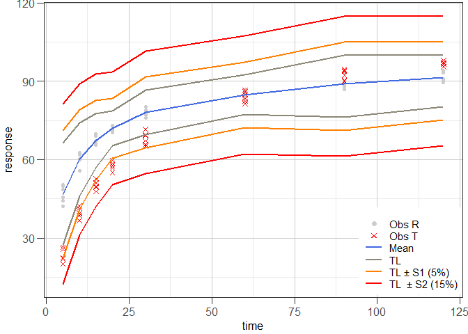
Example 4 illustrates tolerance interval approach proposed by Martinez & Zhao (2018) using the data set that was used in Example 1.
library(disprofas)

# Data frame
str(dip1)
#> 'data.frame':    12 obs. of  10 variables:
#>  $ type  : Factor w/ 2 levels "R","T": 1 1 1 1 1 1 2 2 2 2 ...
#>  $ tablet: Factor w/ 6 levels "1","2","3","4",..: 1 2 3 4 5 6 1 2 3 4 ...
#>  $ t.5   : num  42.1 44.2 45.6 48.5 50.5 ...
#>  $ t.10  : num  59.9 60.2 55.8 60.4 61.8 ...
#>  $ t.15  : num  65.6 67.2 65.6 66.5 69.1 ...
#>  $ t.20  : num  71.8 70.8 70.5 73.1 72.8 ...
#>  $ t.30  : num  77.8 76.1 76.9 78.5 79 ...
#>  $ t.60  : num  85.7 83.3 83.9 85 86.9 ...
#>  $ t.90  : num  93.1 88 86.8 88 89.7 ...
#>  $ t.120 : num  94.2 89.6 90.1 93.4 90.8 ...

# Perform estimation and print a summary
res4 <- mztia(data = dip1, shape = "wide", tcol = 3:10, grouping = "type",
                reference = "R")

class(res4)
#> [1] "mztia"
summary(res4)
#>
#> Results of Martinez & Zhao Tolerance Interval (TI) Approach
#> (TI limits calculated at each time point of the dissolution profiles of a set of reference batches)
#>
#>   Time     Mean      LTL       UTL   S1.LTL    S1.UTL   S2.LTL    S2.UTL
#> 1    5 46.77167 27.22641  66.31693 22.22641  71.31693 12.22641  81.31693
#> 2   10 60.13333 46.15483  74.11184 41.15483  79.11184 31.15483  89.11184
#> 3   15 67.27500 56.90417  77.64583 51.90417  82.64583 41.90417  92.64583
#> 4   20 71.98667 65.44354  78.52979 60.44354  83.52979 50.44354  93.52979
#> 5   30 78.07000 69.54259  86.59741 64.54259  91.59741 54.54259 101.59741
#> 6   60 84.81667 77.20275  92.43058 72.20275  97.43058 62.20275 107.43058
#> 7   90 89.09333 76.24588 100.00000 71.24588 105.00000 61.24588 115.00000
#> 8  120 91.43833 80.29321 100.00000 75.29321 105.00000 65.29321 115.00000
#>
#> Abbreviations:
#> TL: Tolerance Interval Limit (TL); LTL: lower TL; UTL: upper TL; S1: level 1 boundary (LTL - 5) or (UTL + 5); S2: level 2 boundary (LTL - 15) or (UTL + 15).

# Prepare graphical representation
ggres4 <- plot_mztia(res4)
class(ggres4)
#> [1] "plot_mztia"
plot(ggres4)
Pius Dahinden, Tillotts Pharma AG