Implementation of Frequent-Directions algorithm for efficient matrix sketching [E. Liberty, SIGKDD2013]
# Not yet onCRAN
install.packages("frequentdirections")

# Or the development version from GitHub:
install.packages("devtools")
devtools::install_github("shinichi-takayanagi/frequentdirections")Here, we use Handwritten digits USPS dataset as sample data. In the following example, we assume that you save the above sample data into /tmp directory.
The dataset has 7291 train and 2007 test images in h5 format. The images are 16*16 grayscale pixels.
library("h5")
file <- h5file("/tmp/usps.h5")
x <- file["train/data"][]
y <- file["train/target"][]
str(x)
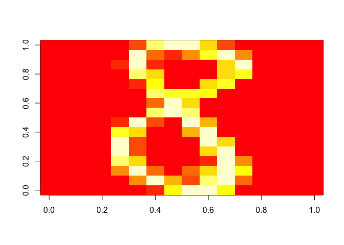
#> num [1:7291, 1:256] 0 0 0 0 0 0 0 0 0 0 ...Example the number 8

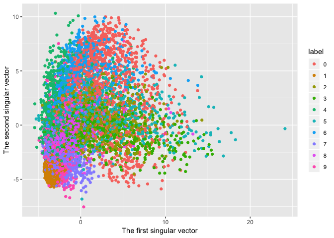
Plot the original data on the first and second singular vector plane.

eps <- 10^(-8)
# 7291 x 256 -> 8 * 256 matrix
b <- frequentdirections::sketching(x, 8, eps)
frequentdirections::plot_svd(x, y, b)
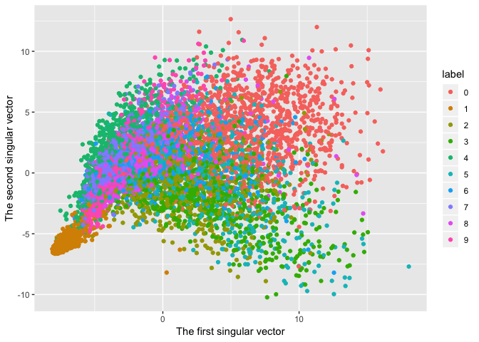
# 7291 x 256 -> 32 * 256 matrix
b <- frequentdirections::sketching(x, 32, eps)
frequentdirections::plot_svd(x, y, b)
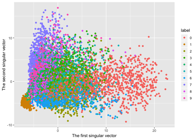
# 7291 x 256 -> 128 * 256 matrix
b <- frequentdirections::sketching(x, 128, eps)
frequentdirections::plot_svd(x, y, b)
This result is almost the same with the original data SVD expression.
That’s why we can think that the original data is expressed with only 128 rows.