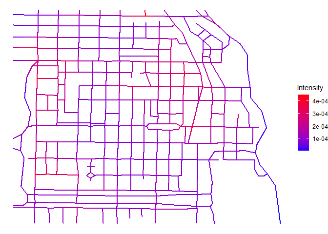
The goal of geonet is to provide a tool for the estimation of the intensity function of a spatial point process on a geometric network. It makes use of generalized additive model (GAM) theory and has a similar workaround. In comparison to other methods, it allows to include external and internal covariates in the model, see the example below.
You can install the released version of geonet from CRAN with:
install.packages("geonet")And the development version from GitHub with:
# install.packages("devtools")
devtools::install_github("MarcSchneble/geonet")This is a basic example which shows you how to solve a common problem:
library(geonet)
library(spatstat.data)

X <- as_gnpp(chicago)
delta <- 10
formula <- X ~ marks + x + y

model <- intensity_pspline(X, formula = formula, delta = delta,
                           scale = list(x = 1/1000, y = 1/1000))
summary(model)
#> Intensity estimation on a geometric network in 2 dimensions
#> with 287 vertices and 452 curve segments.
#> Log-linear Poisson model fitted with maximum likelihood.
#>
#> Global knot distance: 10
#> Global bin width: 5
#>
#> Formula: ~marks + x + y
#>
#> Pparametric coefficients:
#>               Estimate Std. Error z value Pr(>|z|)
#> marksburglary -1.38629    0.50000 -2.7726 0.005561 **
#> markscartheft -1.04982    0.43915 -2.3906 0.016823 *
#> marksdamage    0.55962    0.28030  1.9965 0.045884 *
#> marksrobbery  -1.60944    0.54772 -2.9384 0.003299 **
#> markstheft     0.64185    0.27625  2.3234 0.020156 *
#> markstrespass -1.20397    0.46547 -2.5866 0.009694 **
#> x              0.11757    1.07758  0.1091 0.913119
#> y              1.77584    1.13763  1.5610 0.118524
#> ---
#> Signif. codes:  0 '***' 0.001 '**' 0.01 '*' 0.05 '.' 0.1 ' ' 1
#>
#> Effective degrees of freedom of the baseline intensity: 37.342
#>
#> Number of Fellner-Schall-iterations: 13
plot(model)