
Lüdecke D (2018). ggeffects: Tidy Data Frames of Marginal Effects from Regression Models. Journal of Open Source Software, 3(26), 772. doi: 10.21105/joss.00772
Results of regression models are typically presented as tables that are easy to understand. For more complex models that include interaction or quadratic / spline terms, tables with numbers are less helpful and difficult to interpret. In such cases, marginal effects or adjusted predictions are far easier to understand. In particular, the visualization of such effects or predictions allows to intuitively get the idea of how predictors and outcome are associated, even for complex models.
ggeffects is a light-weight package that aims at easily calculating marginal effects and adjusted predictions (or: estimated marginal means) at the mean or at representative values of covariates (see definitions here) from statistical models, i.e. predictions generated by a model when one holds the non-focal variables constant and varies the focal variable(s). This is achieved by three core ideas that describe the philosophy of the function design:
Functions are type-safe and always return a data frame with the same, consistent structure;
there is a simple, unique approach to calculate marginal effects/adjusted predictions and estimated marginal means for many different models;
the package supports “labelled data” (Lüdecke 2018), which allows human readable annotations for graphical outputs.
This means, users do not need to care about any expensive steps after
modeling to visualize the results. The returned as data frame is ready
to use with the ggplot2-package, however, there is also
a plot()-method to easily create publication-ready
figures.
There is no common language across fields regarding a unique meaning
of “marginal effects.” Thus, the wording throughout this package may
vary. Maybe “adjusted predictions” comes closest to what
ggeffects actually does. To avoid confusion about what
is actually calculated and returned by the package’s functions
ggpredict(), ggemmeans() and
ggeffect(), it is recommended to read this
vignette about the different terminology and its meanings.
Please visit https://strengejacke.github.io/ggeffects/ for documentation and vignettes. For questions about the functionality, you may either contact me via email or also file an issue.
Marginal effects and adjusted predictions can be calculated for many
different models. Currently supported model-objects are:
averaging, bamlss, bayesx,
betabin, betareg, bglmer,
blmer, bracl, brglm,
brmsfit, brmultinom, cgam,
cgamm, clm, clm2,
clmm, coxph, fixest,
gam (package mgcv), Gam
(package gam), gamlss, gamm,
gamm4, gee, geeglm,
glm, glm.nb, glmer,
glmer.nb, glmmTMB, glmmPQL,
glmrob, glmRob, glmx,
gls, hurdle, ivreg,
lm, lm_robust, lme,
lmer, lmrob, lmRob,
logistf, lrm, mclogit,
mlogit, MixMod, MCMCglmm,
mixor, multinom, negbin,
nlmer, ols, orm,
plm, polr, rlm,
rlmer, rq, rqss,
stanreg, survreg, svyglm,
svyglm.nb, tidymodels, tobit,
truncreg, vgam, wbm,
zeroinfl and zerotrunc.
Support for models varies by function, i.e. although
ggpredict(), ggemmeans() and
ggeffect() support most models, some models are only
supported exclusively by one of the three functions. Other models not
listed here might work as well, but are currently not tested.
Interaction terms, splines and polynomial terms are also supported.
The main functions are ggpredict(),
ggemmeans() and ggeffect(). There is a generic
plot()-method to plot the results using
ggplot2.
The returned data frames always have the same, consistent structure
and column names, so it’s easy to create ggplot-plots without the need
to re-write the function call. x and predicted
are the values for the x- and y-axis. conf.low and
conf.high could be used as ymin and
ymax aesthetics for ribbons to add confidence bands to the
plot. group can be used as grouping-aesthetics, or for
faceting.
ggpredict() requires at least one, but not more than
four terms specified in the terms-argument. Predicted
values of the response, along the values of the first term are
calculated, optionally grouped by the other terms specified in
terms.
library(ggeffects)
library(splines)
data(efc)
fit <- lm(barthtot ~ c12hour + bs(neg_c_7) * c161sex + e42dep, data = efc)

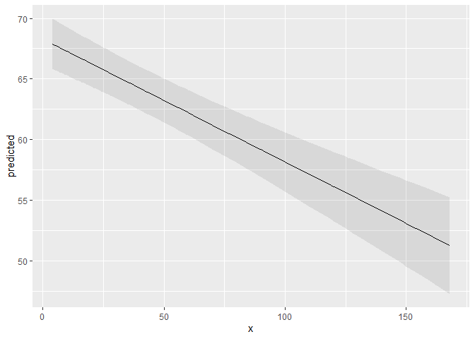
ggpredict(fit, terms = "c12hour")
#> # Predicted values of Total score BARTHEL INDEX
#>
#> c12hour | Predicted |         95% CI
#> ------------------------------------
#>       4 |     67.89 | [65.81, 69.96]
#>      12 |     67.07 | [65.10, 69.05]
#>      22 |     66.06 | [64.19, 67.94]
#>      36 |     64.64 | [62.84, 66.45]
#>      49 |     63.32 | [61.51, 65.14]
#>      70 |     61.20 | [59.22, 63.17]
#>     100 |     58.15 | [55.71, 60.60]
#>     168 |     51.26 | [47.27, 55.25]
#>
#> Adjusted for:
#> * neg_c_7 = 11.83
#> * c161sex =  1.76
#> *  e42dep =  2.93
A possible call to ggplot could look like this:
library(ggplot2)
mydf <- ggpredict(fit, terms = "c12hour")
ggplot(mydf, aes(x, predicted)) +
  geom_line() +
  geom_ribbon(aes(ymin = conf.low, ymax = conf.high), alpha = .1)
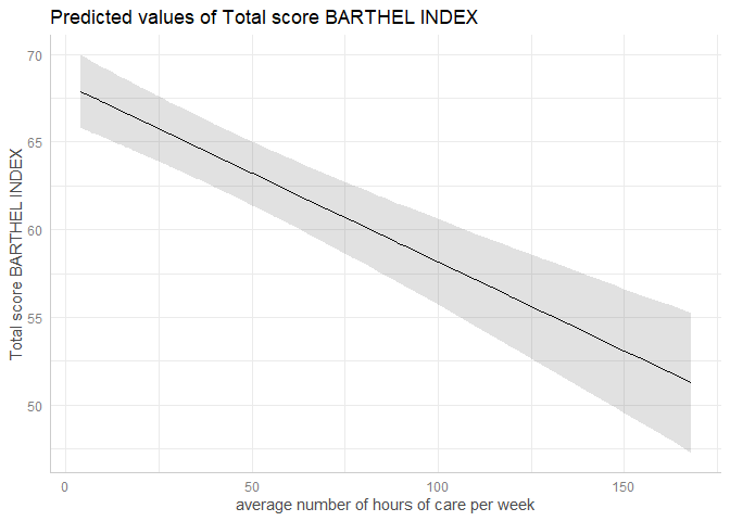
However, there is also a plot()-method. This method uses
convenient defaults, to easily create the most suitable plot for the
marginal effects.
mydf <- ggpredict(fit, terms = "c12hour")
plot(mydf)
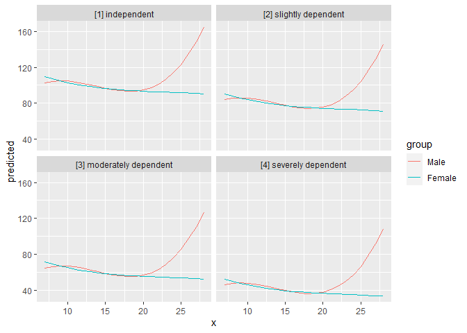
With three variables, predictions can be grouped and faceted.
ggpredict(fit, terms = c("neg_c_7", "c161sex", "e42dep"))
#> # Predicted values of Total score BARTHEL INDEX
#>
#> # c161sex = Male
#> #  e42dep = [1] independent
#>
#> neg_c_7 | Predicted |          95% CI
#> -------------------------------------
#>       7 |    102.74 | [95.97, 109.51]
#>      12 |    102.27 | [97.10, 107.44]
#>      17 |     93.79 | [86.96, 100.63]
#>      28 |    164.57 | [95.98, 233.17]
#>
#> # c161sex = Female
#> #  e42dep = [1] independent
#>
#> neg_c_7 | Predicted |           95% CI
#> --------------------------------------
#>       7 |    109.54 | [105.20, 113.87]
#>      12 |     99.81 | [ 95.94, 103.68]
#>      17 |     94.90 | [ 90.21,  99.60]
#>      28 |     90.26 | [ 71.79, 108.74]
#>
#> # c161sex = Male
#> #  e42dep = [2] slightly dependent
#>
#> neg_c_7 | Predicted |          95% CI
#> -------------------------------------
#>       7 |     83.73 | [77.32,  90.14]
#>      12 |     83.26 | [78.95,  87.58]
#>      17 |     74.79 | [68.68,  80.89]
#>      28 |    145.57 | [77.00, 214.14]
#>
#> # c161sex = Female
#> #  e42dep = [2] slightly dependent
#>
#> neg_c_7 | Predicted |         95% CI
#> ------------------------------------
#>       7 |     90.53 | [86.71, 94.35]
#>      12 |     80.80 | [78.17, 83.44]
#>      17 |     75.90 | [72.29, 79.51]
#>      28 |     71.26 | [53.07, 89.45]
#>
#> # c161sex = Male
#> #  e42dep = [3] moderately dependent
#>
#> neg_c_7 | Predicted |          95% CI
#> -------------------------------------
#>       7 |     64.72 | [58.28,  71.16]
#>      12 |     64.26 | [60.30,  68.21]
#>      17 |     55.78 | [50.04,  61.52]
#>      28 |    126.56 | [57.98, 195.14]
#>
#> # c161sex = Female
#> #  e42dep = [3] moderately dependent
#>
#> neg_c_7 | Predicted |         95% CI
#> ------------------------------------
#>       7 |     71.52 | [67.59, 75.45]
#>      12 |     61.79 | [59.79, 63.80]
#>      17 |     56.89 | [53.86, 59.91]
#>      28 |     52.25 | [34.21, 70.29]
#>
#> # c161sex = Male
#> #  e42dep = [4] severely dependent
#>
#> neg_c_7 | Predicted |          95% CI
#> -------------------------------------
#>       7 |     45.72 | [38.86,  52.57]
#>      12 |     45.25 | [41.03,  49.47]
#>      17 |     36.77 | [30.97,  42.58]
#>      28 |    107.55 | [38.93, 176.18]
#>
#> # c161sex = Female
#> #  e42dep = [4] severely dependent
#>
#> neg_c_7 | Predicted |         95% CI
#> ------------------------------------
#>       7 |     52.51 | [47.88, 57.15]
#>      12 |     42.79 | [40.29, 45.28]
#>      17 |     37.88 | [34.66, 41.10]
#>      28 |     33.24 | [15.21, 51.28]
#>
#> Adjusted for:
#> * c12hour = 42.10

mydf <- ggpredict(fit, terms = c("neg_c_7", "c161sex", "e42dep"))
ggplot(mydf, aes(x = x, y = predicted, colour = group)) +
  geom_line() +
  facet_wrap(~facet)
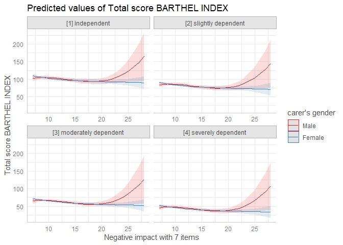
plot() works for this case, as well:
plot(mydf)
More features are explained in detail in the package-vignettes.
To install the latest development snapshot (see latest changes below), type following commands into the R console:
library(devtools)
devtools::install_github("strengejacke/ggeffects")To install the latest stable release from CRAN, type following command into the R console:
install.packages("ggeffects")In case you want / have to cite my package, please use
citation('ggeffects') for citation information:
Lüdecke D (2018). ggeffects: Tidy Data Frames of Marginal Effects from Regression Models. Journal of Open Source Software, 3(26), 772. doi: 10.21105/joss.00772