InteractionR allows researchers to produce publication-ready tables that includes all effect estimates necessary for full reporting effect modification and interaction analysis as recommended by Knol and Vanderweele (2012) (doi:10.1093/ije/dyr218). It also estimates confidence interval for the trio of additive interaction measures using the delta method (Hosmer and Lemeshow (1992), doi:10.1097/00001648-199209000-00012), variance recovery method (Zou (2008), doi:10.1093/aje/kwn104), or percentile bootstrapping (Assmann et al. (1996), doi:10.1097/00001648-199605000-00012).
interactionR is on CRAN, install
using install.packages("interactionR").
You can also install the development version from GitHub with:
# install.packages("devtools")
devtools::install_github("epi-zen/interactionR")interactionR is implemented in the R statistical software
environment; R is installable from https://www.r-project.org/. The main user-facing
function of the package, interactionR(), accepts the
following arguments:
model: a regression model fitted by the user with interaction term for the two exposures under consideration. This may be an object of class glm with a valid link for logistic regression or approximants of risk ratio, class clogit or class coxph. It can also include confounders adjustment as is usually the case.
exposure_names: A character vector of two named binary exposure variables present in the fitted model.
ci.type: A character string (“delta” or “mover”) specifying the method to use for the estimation of CI for the measures of additive interaction. Default is “delta”.
ci.level: Magnitude of the returned CI level.
em: TRUE, for effect modification assessment. FALSE, for interaction.
recode: If TRUE, recodes the exposures - if at least one of the exposures is protective - such that the stratum with the lowest risk becomes the new reference category when the two exposures are considered jointly (See Knol et al (2011) [doi: 10.1007/s10654-011-9554-9]).
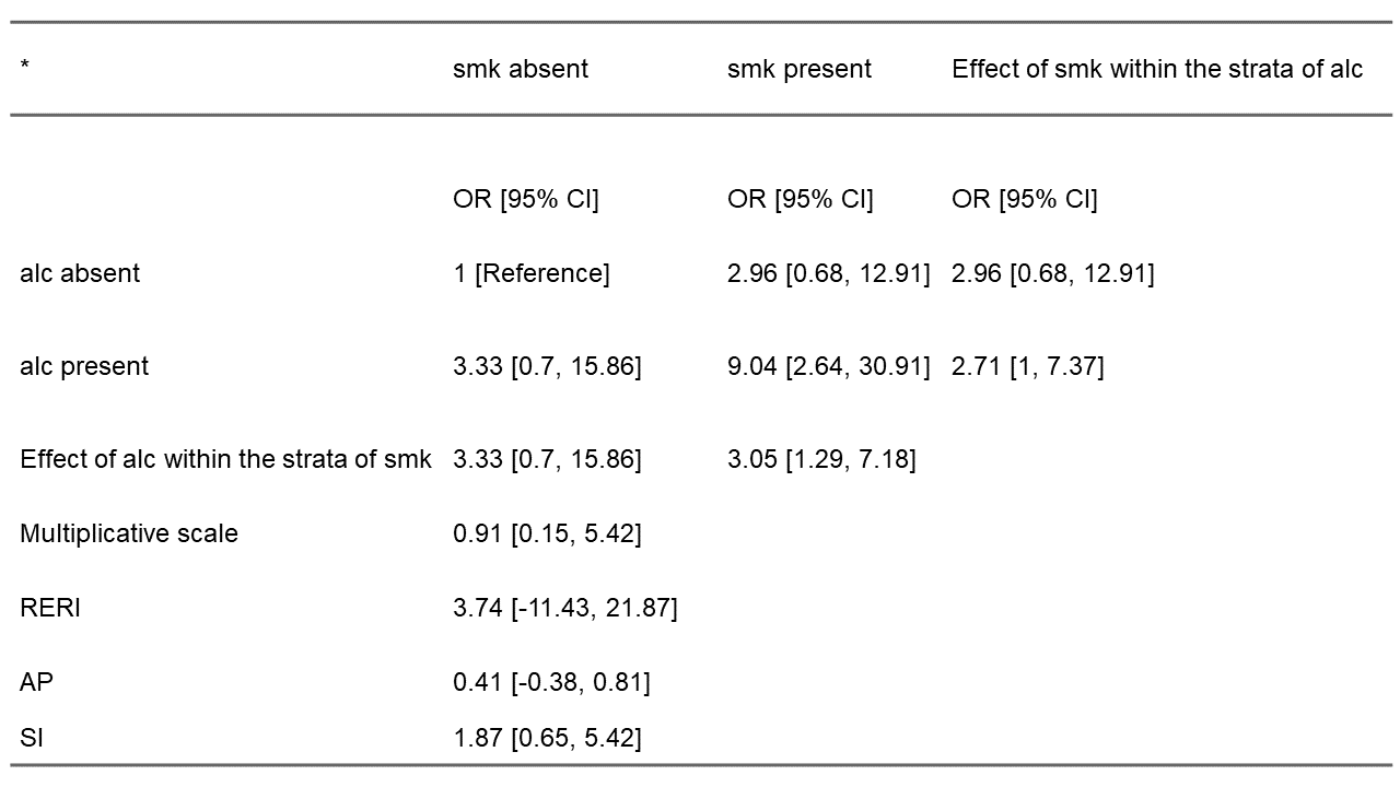
Consider the case-control data from Rothman and Keller (1979) [doi: 10.1016/0021-9681(72)90006-9], which studied the joint effect of alcohol and smoking on oral cancers. This dataset was used previously by Hosmer and Lemeshow, and Zou and its included in our package as ‘OCdata’ for easy replication of our analysis by the user. It contains the two exposures, alcohol (‘alc’) and smoking (‘smk’), and the outcome, oral cancer (‘oc’) as dichotomous variables (0 or 1, indicating absence or presence respectively). Suppose we are considering interaction and we want to compute the CIs for the measures of additive interaction using the MOVER method, we will start by fitting the following logistic regression model with an interaction term for alcohol and smoking on oral cancer:
library(interactionR)
data (OCdata)

## fit the interaction model
model.glm <- glm(oc ~ alc*smk, family = binomial(link = "logit"), data = OCdata)
Then, pass the fitted model to the function which generates a list object of class ‘interactionR’
table_object = interactionR(model.glm, exposure_names = c("alc", "smk"), ci.type = "mover", ci.level = 0.95, em = F, recode = F)This returns a list object of class interactionR which includes a
dataframe containing all the effect estimates that are necessary to
fully report effect modification or interaction. This data frame and
other components of the list are accessible to the user for further
manipulation, if desired. Importantly, the output object is formatted in
such a way that the data frame can be processed by the tabling function
interactionR_table(). An example is:
interactionR_table(table_object)
The tabling function will generate and save a publication-ready table
as a word document to the user’s working directory, if desired. The
returned point estimate and CI for RERI (3.74; 95% CI: -11.43, 21.87) is
as reported by Zou for this data (13) – If the ‘ci.type’ argument in the
interactionR() call had been set to “delta”, the CIs for
this trio of interaction measures would be as reported by Hosmer and
Lemeshow.
In addition to the main function described above, the package also provides standalone functions for each of the CI estimating methods: interactionR_mover(), interactionR_delta(), and interactionR_boot(). The latter implements the percentile bootstrapping of CIs of additive interaction measures as described by Assmann et al, with usage shown in the next example.
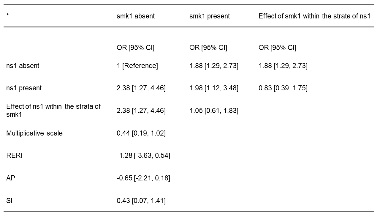
To illustrate the interactionR_boot() function, consider the case-control data of the effect of sports participation and smoking on herniated lumbar disc examined by Assmann et al. in their analysis. The dataset is available in the package as ‘HDiscdata’ and contains three binary variables: i) the outcome. herniated lumbar disc, ‘h’; and ii & iii) the exposures sports participation, ‘ns’, and smoking ‘smk’. The function accepts the following arguments:
model: A fitted model of class glm. Requires the exposures with interaction term to be listed first before any other covariates/confounders (if applicable).
ci.level; em; recode: As previously
described for interactionR().
seed: The random number seed to use for generating the bootstrap samples (for reproducibility). Default is 12345 but can be set to any number.
s: Number of bootstrap resampling. Default is 1000
Again, we start by fitting a logistic regression model:
data(HDiscdata)
m2 = glm(h ~ ns*smk, family = binomial(link = 'logit'), data = HDiscdata)
Then, pass the object to the interactionR_boot()
function as follows:
table_object2 = interactionR_boot(m2, ci.level = 0.95, em = F, recode = F, seed = 12345, s = 1000)Loading required namespace: bootThis runs a non-parametric bootstrap sample 1000 times with
replacements and a percentile CI. The function also returns a list
object of class interactionR containing all the desired estimates and
manipulable by the tabling function - interactionR_table()
- described earlier. Calling interactionR_table() on the
returned object produces a publication-ready table with estimates for
the CI of RERI and AP similar to that reported by Assmann et al. for
this data.
interactionR_table(table_object2) Furthermore, some
base R functions are available to the user to further manipulate some
parts of the output object from interactionR_boot(). A simple example
is:
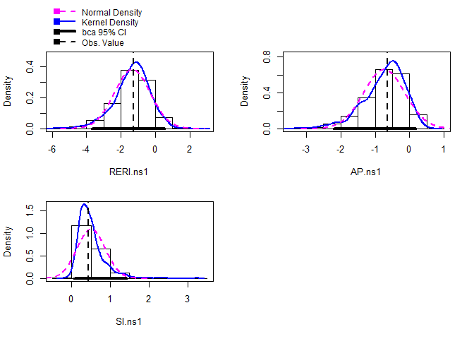
hist(table_object2$bootstrap)
This produce histograms of the distribution of each of the three bootstrapped parameters (RERI, AP and SI), allowing the user to inspect the overall performance and accuracy of the returned estimates.
Cite as: Babatunde Y. Alli (2021). InteractionR: An R package for full reporting of effect modification and interaction. Software Impacts, 10, 100147. doi:10.1016/j.simpa.2021.100147
For contribute to interactionR please feel free to fork the branch and send me pull requests. Currently, only the master branch is used for both development and releases.
Please use interactionR issues here on Github.
Please consult the help files for the package within R or contact the maintainer at babatunde.alli [at] mail.mcgill.ca