The goal of nlmixr2 is to support easy and robust nonlinear mixed effects models in R
For all versions of R, we need to have a compiler setup to run
nlmixr2 and rxode2
For Windows the compilers come from Rtools. For R version 4.2 and above you need to have Rtools42, for R-4.0.x, and R-4.1.x you need Rtools40. Download and the install from https://cran.r-project.org/bin/windows/Rtools/
To setup the mac compilers, simply
Install Xcode from app store
Install gfortran:
Download and install from https://mac.r-project.org/tools/
Add gfortran directory to the path with:
export PATH=$PATH:/usr/local/gfortran/bin
Installation nlmixr2 itself is easiest in R-4.2.x because no further compilation is required and all supporting packages are available. From R, run:
install.packages("nlmixr2",dependencies = TRUE)For R-4.0.x and R-4.1.x, the crucial package symengine is currently not on CRAN and will have to be installed from MRAN first by running:
install.packages("symengine", repos="https://cran.microsoft.com/snapshot/2022-01-01/")followed by:
install.packages("nlmixr2",dependencies = TRUE)Once the compilers are setup and a compatible version of
symengine is installed, you can install the development
version of nlmixr2 and its nlmixr2-family dependencies like so:
remotes::install_github("nlmixr2/nlmixr2data")
remotes::install_github("nlmixr2/lotri")
remotes::install_github("nlmixr2/rxode2")
remotes::install_github("nlmixr2/nlmixr2est")
remotes::install_github("nlmixr2/nlmixr2extra")
remotes::install_github("nlmixr2/nlmixr2plot")
remotes::install_github("nlmixr2/nlmixr2")
Optional supporting packages can be installed like so:
remotes::install_github("ggPMXdevelopment/ggPMX") # Goodness of fit plots
remotes::install_github("nlmixr2/xpose.nlmixr2") # Additional goodness of fit plots
remotes::install_github("RichardHooijmaijers/shinyMixR") # Shiny run manager (like Piranha)
remotes::install_github("nlmixr2/nlmixr2targets") # Simplify work with the `targets` package
If you have difficulties due to errors while compiling models, it may
be useful to reinstall all of nlmixr2 and its dependencies. For
development versions, please use the
remotes::install_github() commands above. For the stable
version, please use the following command:
install.packages(c("nlmixr2", "nlmixr2est", "rxode2", "nlmixr2plot", "nlmixr2data", "lotri", "nlmixr2extra"))This is a basic example which shows you how to solve a common problem:
library(nlmixr2)

## The basic model consiss of an ini block that has initial estimates
one.compartment <- function() {
  ini({
    tka <- 0.45 # Log Ka
    tcl <- 1 # Log Cl
    tv <- 3.45    # Log V
    eta.ka ~ 0.6
    eta.cl ~ 0.3
    eta.v ~ 0.1
    add.sd <- 0.7
  })
  # and a model block with the error sppecification and model specification
  model({
    ka <- exp(tka + eta.ka)
    cl <- exp(tcl + eta.cl)
    v <- exp(tv + eta.v)
    d/dt(depot) = -ka * depot
    d/dt(center) = ka * depot - cl / v * center
    cp = center / v
    cp ~ add(add.sd)
  })
}

## The fit is performed by the function nlmixr/nlmix2 specifying the model, data and estimate
fit <- nlmixr2(one.compartment, theo_sd,  est="saem", saemControl(print=0))
#>
#>
#>
#> ℹ parameter labels from comments will be replaced by 'label()'
#>
#> → loading into symengine environment...
#> → pruning branches (`if`/`else`) of saem model...
#> ✔ done
#> → finding duplicate expressions in saem model...
#> → optimizing duplicate expressions in saem model...
#> ✔ done
#> rxode2 2.0.7 model named rx_7bde54c6c90c8ab16296ac0ee0a3a632 model (✔ ready).
#> $state: depot, center
#> $stateExtra: cp
#> $params: tka, tcl, tv
#> $lhs: rx_pred_
#> Calculating covariance matrix
#> rxode2 2.0.7 model named rx_7bde54c6c90c8ab16296ac0ee0a3a632 model (✔ ready).
#> $state: depot, center
#> $stateExtra: cp
#> $params: tka, tcl, tv
#> $lhs: rx_pred_
#> rxode2 2.0.7 model named rx_7bde54c6c90c8ab16296ac0ee0a3a632 model (✔ ready).
#> $state: depot, center
#> $stateExtra: cp
#> $params: tka, tcl, tv
#> $lhs: rx_pred_
#> rxode2 2.0.7 model named rx_7bde54c6c90c8ab16296ac0ee0a3a632 model (✔ ready).
#> $state: depot, center
#> $stateExtra: cp
#> $params: tka, tcl, tv
#> $lhs: rx_pred_
#> rxode2 2.0.7 model named rx_7bde54c6c90c8ab16296ac0ee0a3a632 model (✔ ready).
#> $state: depot, center
#> $stateExtra: cp
#> $params: tka, tcl, tv
#> $lhs: rx_pred_
#> → loading into symengine environment...
#> → pruning branches (`if`/`else`) of saem model...
#> ✔ done
#> → finding duplicate expressions in saem predOnly model 0...
#> → finding duplicate expressions in saem predOnly model 1...
#> → optimizing duplicate expressions in saem predOnly model 1...
#> → finding duplicate expressions in saem predOnly model 2...
#> ✔ done
#>
#> → Calculating residuals/tables
#> ✔ done
#> → compress origData in nlmixr2 object, save 5952
#> → compress phiM in nlmixr2 object, save 62360
#> → compress parHist in nlmixr2 object, save 9560
#> → compress saem0 in nlmixr2 object, save 23224
print(fit)
#> ── nlmixr SAEM OBJF by FOCEi approximation ──
#>
#>  Gaussian/Laplacian Likelihoods: AIC() or $objf etc.
#>  FOCEi CWRES & Likelihoods: addCwres()
#>
#> ── Time (sec $time): ──
#>
#>            setup covariance  saem table compress    other
#> elapsed 0.001214   0.087003 2.579 0.018    0.024 0.830783
#>
#> ── Population Parameters ($parFixed or $parFixedDf): ──
#>
#>        Parameter  Est.     SE %RSE Back-transformed(95%CI) BSV(CV%) Shrink(SD)%
#> tka       Log Ka 0.454  0.196 43.1       1.57 (1.07, 2.31)     71.5   -0.0203%
#> tcl       Log Cl  1.02 0.0853  8.4       2.76 (2.34, 3.26)     27.6      3.46%
#> tv         Log V  3.45 0.0454 1.32       31.5 (28.8, 34.4)     13.4      9.89%
#> add.sd           0.693                               0.693
#>
#>   Covariance Type ($covMethod): linFim
#>   No correlations in between subject variability (BSV) matrix
#>   Full BSV covariance ($omega) or correlation ($omegaR; diagonals=SDs)
#>   Distribution stats (mean/skewness/kurtosis/p-value) available in $shrink
#>
#> ── Fit Data (object is a modified tibble): ──
#> # A tibble: 132 × 19
#>   ID     TIME    DV  PRED    RES IPRED   IRES  IWRES eta.ka eta.cl   eta.v    cp
#>   <fct> <dbl> <dbl> <dbl>  <dbl> <dbl>  <dbl>  <dbl>  <dbl>  <dbl>   <dbl> <dbl>
#> 1 1      0     0.74  0     0.74   0     0.74   1.07   0.103 -0.491 -0.0820  0
#> 2 1      0.25  2.84  3.27 -0.426  3.87 -1.03  -1.48   0.103 -0.491 -0.0820  3.87
#> 3 1      0.57  6.57  5.85  0.723  6.82 -0.246 -0.356  0.103 -0.491 -0.0820  6.82
#> # … with 129 more rows, and 7 more variables: depot <dbl>, center <dbl>,
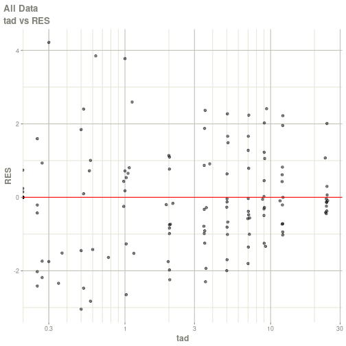
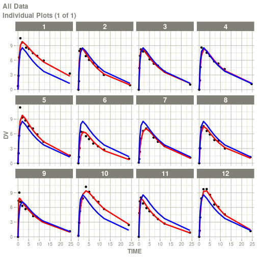
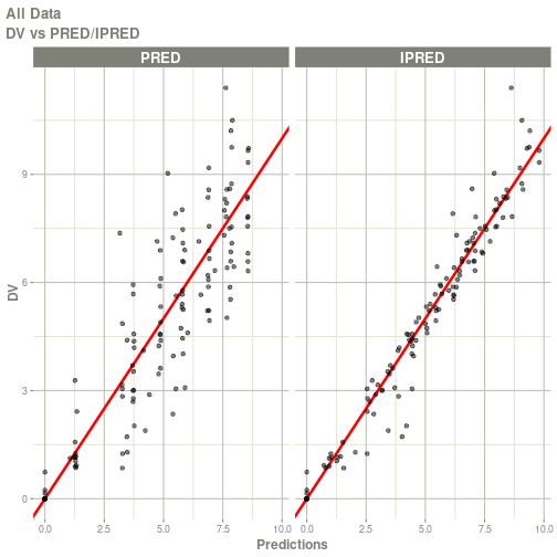
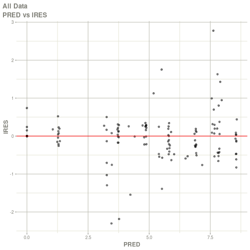
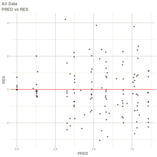
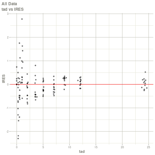
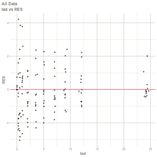
#> # ka <dbl>, cl <dbl>, v <dbl>, tad <dbl>, dosenum <dbl>plot(fit)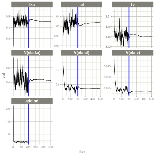
#> Warning: Transformation introduced infinite values in continuous x-axis
#> Warning: Transformation introduced infinite values in continuous y-axis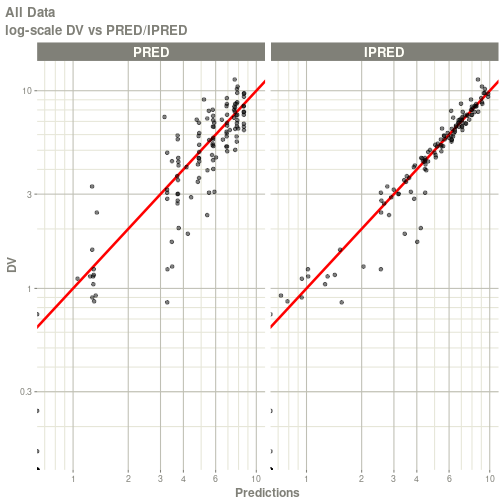
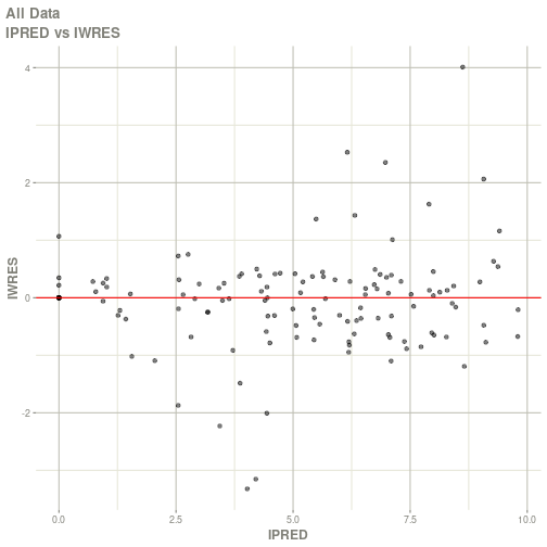
#> Warning: Transformation introduced infinite values in continuous x-axis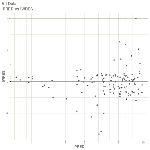
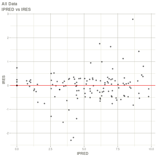
#> Warning: Transformation introduced infinite values in continuous x-axis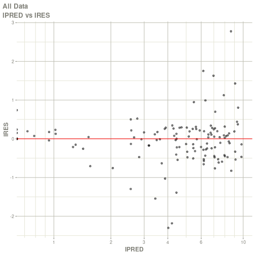
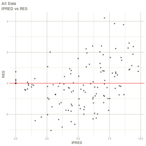
#> Warning: Transformation introduced infinite values in continuous x-axis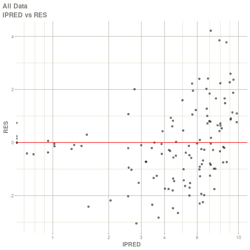
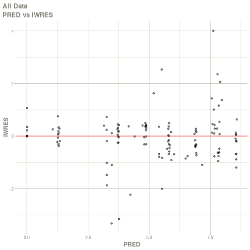
#> Warning: Transformation introduced infinite values in continuous x-axis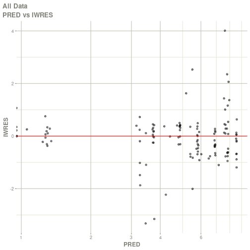
#> Warning: Transformation introduced infinite values in continuous x-axis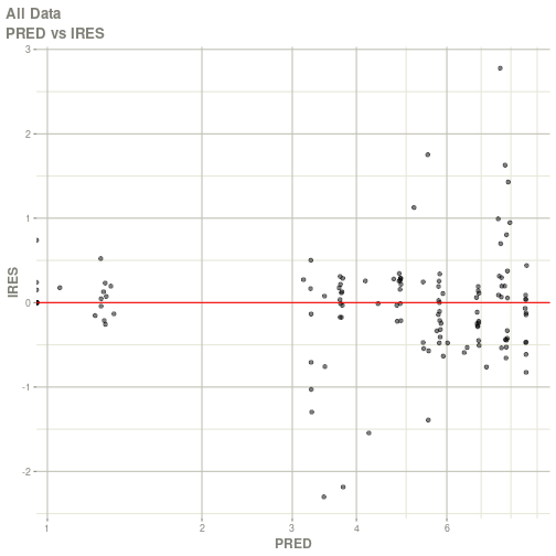
#> Warning: Transformation introduced infinite values in continuous x-axis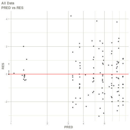
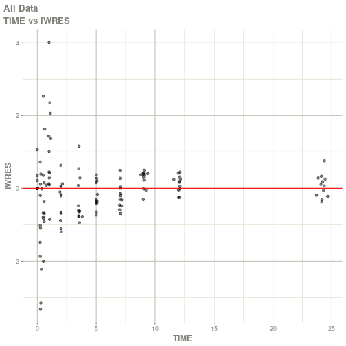
#> Warning: Transformation introduced infinite values in continuous x-axis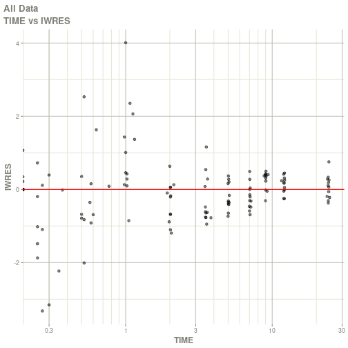
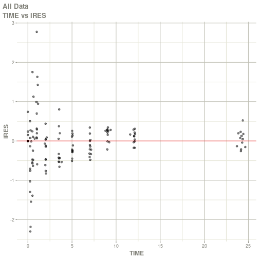
#> Warning: Transformation introduced infinite values in continuous x-axis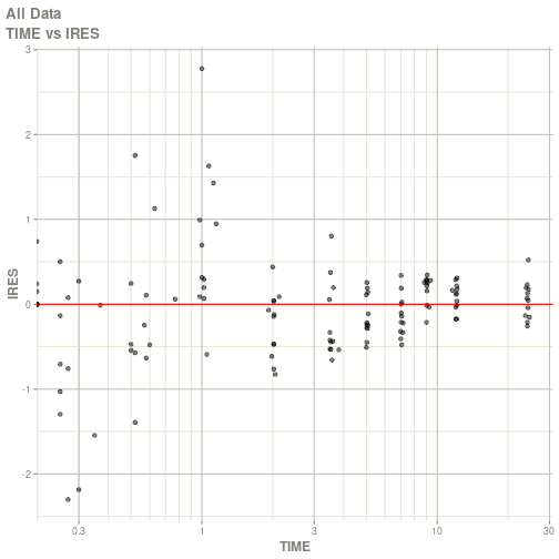
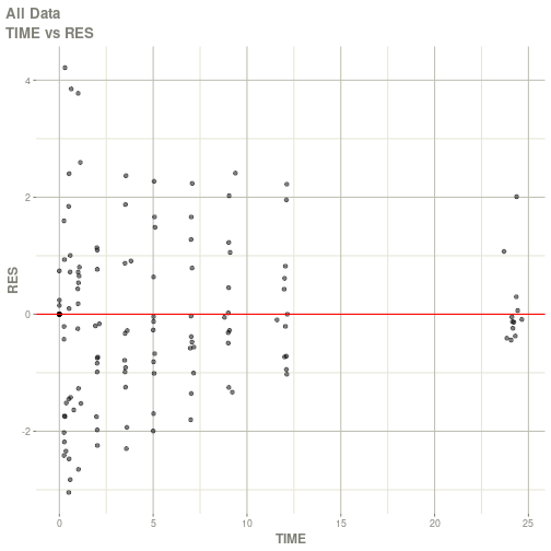
#> Warning: Transformation introduced infinite values in continuous x-axis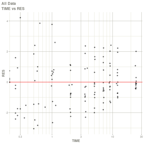
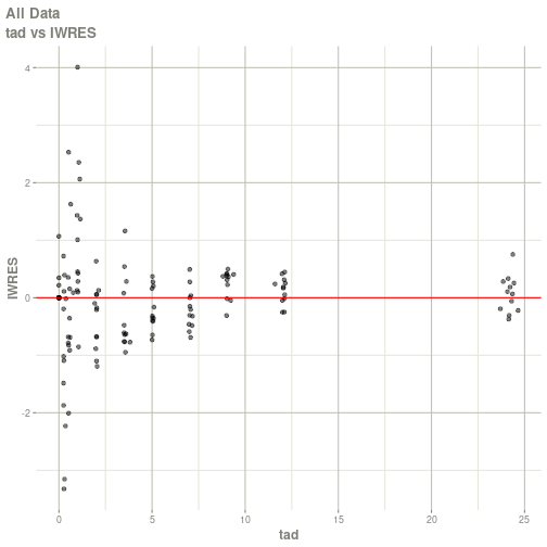
#> Warning: Transformation introduced infinite values in continuous x-axis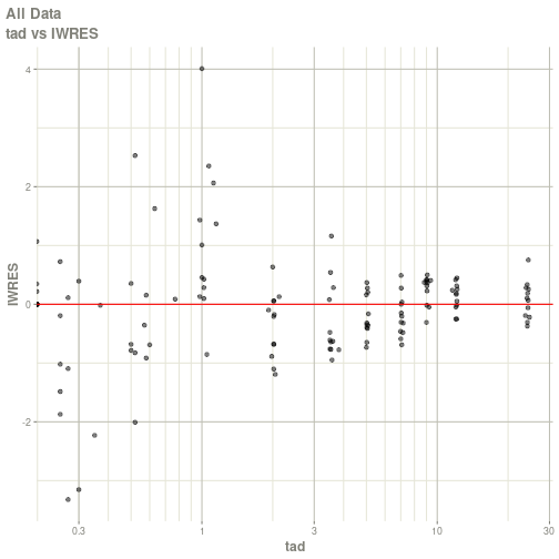
#> Warning: Transformation introduced infinite values in continuous x-axis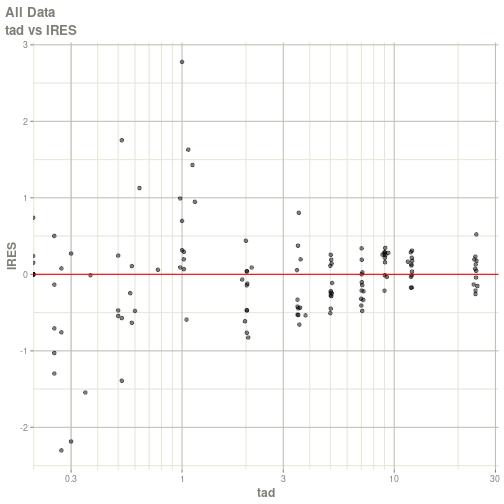
#> Warning: Transformation introduced infinite values in continuous x-axis