The package optedr is an optimal experimental design suite for calculating optimal designs, D-augmenting designs and efficiently rounding approximate design. Among its capabilities are:
You can install the released version of optedr from CRAN with:
You can install the latest version of the package from GitHub with:
The user available functions are:
opt_des() calculates optimal designs.design_efficiency() evaluates the efficiency of a design against the optimum.augment_design() augments designs, allowing the user to add points controlling the D-efficiency.efficient_round() efficiently round approximate designs.shiny_optimal() demo of optimal designs calculation with a graphical interface, applied to Antoine’s Equation.shiny_augment() demo of augmenting design with a graphical interface, usable for a handful of models.The optdes object generated by opt_des() has its own implementation of print(), summary() and plot().
The calculation of an optimal design requires a to specify the Criterion, the model, the parameters and their initial values and the design_space.
resArr.D <- opt_des(Criterion = "D-Optimality",
                    model = y ~ a*exp(-b/x),
                    parameters = c("a", "b"),
                    par_values = c(1, 1500),
                    design_space = c(212, 422))
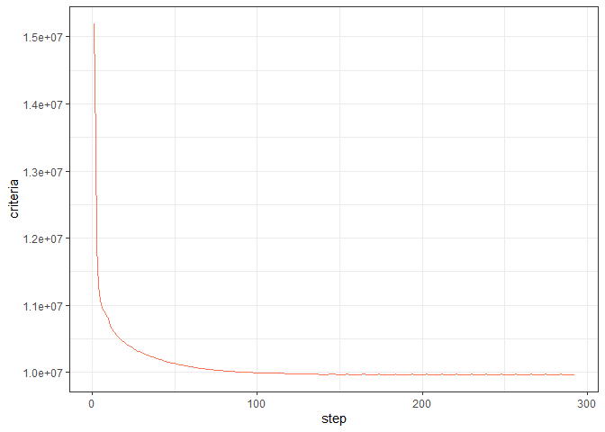
#> i Stop condition not reached, max iterations performed
#> i The lower bound for efficiency is 99.9986396401789%

resArr.D$optdes
#>      Point    Weight
#> 1 329.2966 0.5000068
#> 2 422.0000 0.4999932
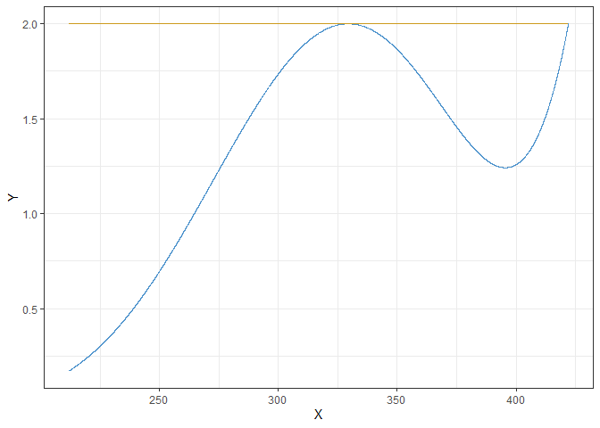
resArr.D$sens

After calculating the D-optimal design, the user might want to add points to the design to fit their needs:
aug_arr <- augment_design(resArr.D$optdes, 0.3, y ~ a * exp(-b/x),
               parameters = c("a", "b"),
               par_values = c(1, 1500),
               design_space = c(212, 422),
               F)
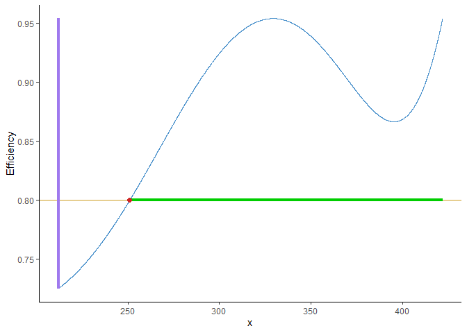
#> The region(s) are  [250.98-422]The region(s) are  [250.98-422]The region(s) are  [250.98-422]
aug_arr
#>      Point    Weight
#> 1 329.2966 0.3500048
#> 2 422.0000 0.3499952
#> 3 260.0000 0.1500000
#> 4 380.0000 0.1500000
This new design can be rounded to the desired number of points:
(exact_design <- efficient_round(aug_arr, 20))
#>      Point Weight
#> 1 329.2966      7
#> 2 422.0000      7
#> 3 260.0000      3
#> 4 380.0000      3
And its efficiency compared against the optimum: