
The goal of ribd is to compute various coefficients of relatedness and identity-by-descent (IBD) between pedigree members. It extends the pedtools package which provides useful utilities for pedigree construction and manipulation.
The main functions in ribd are the following, all of which support both autosomal and X-chromosomal modes:
kinship() : Kinship coefficientsinbreeding() : Inbreeding coefficientskappaIBD() : IBD coefficients kappa = (k0, k1, k2) between noninbred individualsidentityCoefs() : Jacquard’s condensed identity coefficientsA unique feature of ribd is the ability to handle pedigrees with inbred founders in all of the above calculations. More about this below!
The package also computes a variety of lesser-known pedigree coefficients:
gKinship() : Generalised kinship coefficients of various kinds, including those defined by Karigl (1981), Weeks & Lange (1988), Lange & Sinsheimer (1992) and García-Cortés (2015).multiPersonIBD() : Multi-person IBD coefficients (noninbred individuals only)twoLocusKinship() : Two-locus kinship coefficients, as defined by Thompson (1988)twoLocusIBD() : Two-locus IBD coefficients (noninbred pair of individuals)twoLocusIdentity() : Two-locus condensed identity coefficients (any pair of individuals)twoLocusGeneralisedKinship() : Generalised two-locus kinship coefficients (not exported)To get the current official version of ribd, install from CRAN as follows:
Alternatively, you can obtain the latest development version from GitHub:
# install.packages("devtools") # install devtools if needed
devtools::install_github("magnusdv/ribd")In the following we illustrate the use of ribd by computing a few well-known examples. We start by loading the package.
For a child of related parents, its inbreeding coefficient is defined as the probability of autozygosity (i.e., homologous alleles being IBD) in a random autosomal locus.
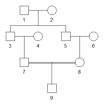
For example, the child of first cousins shown above has inbreeding coefficient 1/16. We can compute this with ribd as follows:
# Create pedigree
x = cousinPed(1, child = TRUE)

# Plot pedigree
plot(x)

# Inbreeding coefficient of the child
inbreeding(x, ids = 9)
#> [1] 0.0625By theory, the above inbreeding coefficient should equal the kinship coefficient between the parents, i.e., the cousins 7 and 8:
As expected, the result was again 1/16.
For a pair of noninbred individuals, the three kappa coefficients are defined as the probability that they have exactly 0, 1 or 2 alleles IBD, respectively, at a random autosomal locus. For example, for a pair of full siblings, this works out to be 1/4, 1/2 and 1/4, respectively.
Since the three kappa’s always sum to 1, any two of them are sufficient, forming the coordinates of a point in the plane. This gives rise to the IBD triangle, which is a useful tools for visualising (noninbred) relationships. The implementation in ribd uses kappa0 on the first axis and kappa2 on the second. In the example below, we place all pairs of pedigree members in the triangle.
We validate this with the kappaIBD() function of ribd:
# Create and plot pedigree
y = nuclearPed(2)
plot(y, margin = rep(4, 4))

# Compute kappa for all pairs
k = kappaIBD(y)

# IBD triangle
showInTriangle(k, labels = T, cexLab = 1.3, pos = c(3,2,3,4,4,3))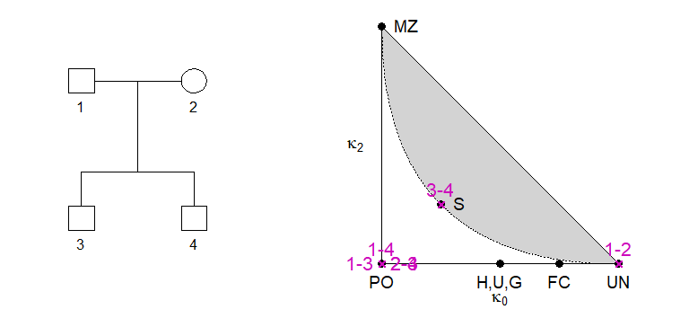
As shown by Thompson (1976), all relationships of noninbred individuals satisfy a certain quadratic inequality in the kappa’s, resulting in an unattainable region of the triangle (shown in grey above).
Here is a relationship in the interior of the attainable region of the IBD triangle:
z = halfSibStack(2)
plot(z, hatched = 7:8, margin = c(3,2,2,2))

kap = kappaIBD(z, ids = 7:8)
showInTriangle(kap)
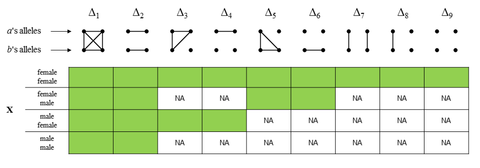
The following figure shows the 9 condensed identity states of two individuals a and b. Each state shows a pattern of identity by descent (IBD) between the four homologous alleles. The four alleles are represented as dots, with a connecting line segment indicating IBD. The states are shown in the ordering used by Jacquard and most subsequent authors.

The following relationship is perhaps the simplest example where all 9 coefficients are nonzero.
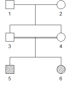
The function identityCoefs() by default returns the nine coefficients in the order given above.
identityCoefs(x, ids = 5:6)
#> [1] 0.06250 0.03125 0.12500 0.03125 0.12500 0.03125 0.21875 0.31250 0.06250The X-chromosomal version of Jacquard’s identity coefficients can be computed by adding Xchrom = TRUE in the call to identityCoefs(). Here is the output for all pairs in the above pedigree:
identityCoefs(x, Xchrom = TRUE)
#>    id1 id2    D1    D2   D3   D4   D5  D6   D7  D8 D9
#> 1    1   2 0.000 0.000 0.00 1.00   NA  NA   NA  NA NA
#> 2    1   3 0.000 1.000   NA   NA   NA  NA   NA  NA NA
#> 3    1   4 0.000 0.000 1.00 0.00   NA  NA   NA  NA NA
#> 4    1   5 0.500 0.500   NA   NA   NA  NA   NA  NA NA
#> 5    1   6 0.000 0.250 0.50 0.25   NA  NA   NA  NA NA
#> 6    2   3 0.000 0.000   NA   NA 1.00 0.0   NA  NA NA
#> 7    2   4 0.000 0.000 0.00 0.00 0.00 0.0 0.00 1.0  0
#> 8    2   5 0.000 0.000   NA   NA 0.50 0.5   NA  NA NA
#> 9    2   6 0.000 0.000 0.00 0.00 0.25 0.0 0.25 0.5  0
#> 10   3   4 0.000 0.000 0.50 0.50   NA  NA   NA  NA NA
#> 11   3   5 0.250 0.750   NA   NA   NA  NA   NA  NA NA
#> 12   3   6 0.250 0.000 0.75 0.00   NA  NA   NA  NA NA
#> 13   4   5 0.000 0.000   NA   NA 1.00 0.0   NA  NA NA
#> 14   4   6 0.000 0.000 0.00 0.00 0.25 0.0 0.25 0.5  0
#> 15   5   6 0.125 0.125 0.50 0.25   NA  NA   NA  NA NA
A precise definition of these X-chromosomal coefficients requires some explanation, which we give here.
As in the autosomal case, the identity coefficients on X are the expected proportions of the possible IBD states involving the alleles at a random locus (on X). The challenge is that the set of states depends on the individual’s sex: F/F, F/M, M/F or M/M (were F = female and M = male). The easiest case is F/F: When both are female, the states are just as in the autosomal case.
Males, being hemizygous, have only 1 allele of a locus on X. Hence when males are involved the total number of alleles is less than 4, rendering the autosomal states pictured above meaningless. However, to avoid drawing (and learning the ordering of) new states for each sex combination, we can re-use the autosomal state pictograms by invoking the following simple rule: Replace the single allele of any male, with a pair of autozygous alleles. This gives a one-to-one map from the X states to the autosomal states.
For simplicity the output always contains 9 coefficients, but with NA’s in the positions of undefined states (depending on the sex combination). Hopefully this should all be clear from the following table:
A unique feature of ribd (in fact, throughout the ped suite packages) is the support for inbred founders. This greatly expands the set of pedigrees we can analyse with a computer.
Here is a fun example using inbred founders: A relationship exactly midway (at least arithmetically speaking) between parent-child and full siblings. To achieve this, we modify the pedigree z from above (half-sibs/half-cousins), giving two of the founders carefully chosen inbreeding coefficients.
Note that founder inbreeding is by default included in the pedigree plot:
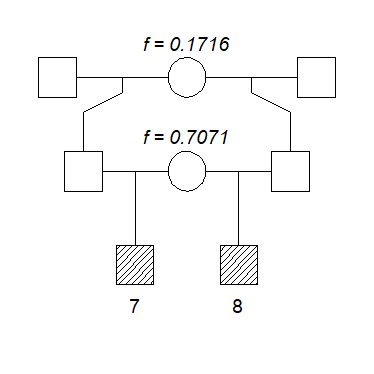
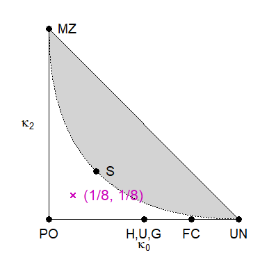
If you wonder how the weird-looking inbreeding coefficients above were chosen, you can check out my paper Relatedness coefficients in pedigrees with inbred founders (J Math Biol, 2020). In it I show that any point in the white region of the IBD triangle can be constructed as a double half cousin relationship with suitable founder inbreeding.
The construction described in the paper is implemented in the function constructPedigree() in ribd. For example, the following command produces basically the pedigree in the previous figure: