shapr

The most common machine learning task is to train a model which is able to predict an unknown outcome (response variable) based on a set of known input variables/features. When using such models for real life applications, it is often crucial to understand why a certain set of features lead to exactly that prediction. However, explaining predictions from complex, or seemingly simple, machine learning models is a practical and ethical question, as well as a legal issue. Can I trust the model? Is it biased? Can I explain it to others? We want to explain individual predictions from a complex machine learning model by learning simple, interpretable explanations.

Shapley values is the only prediction explanation framework with a solid theoretical foundation (Lundberg and Lee (2017)). Unless the true distribution of the features are known, and there are less than say 10-15 features, these Shapley values needs to be estimated/approximated. Popular methods like Shapley Sampling Values (Štrumbelj and Kononenko (2014)), SHAP/Kernel SHAP (Lundberg and Lee (2017)), and to some extent TreeSHAP (Lundberg, Erion, and Lee (2018)), assume that the features are independent when approximating the Shapley values for prediction explanation. This may lead to very inaccurate Shapley values, and consequently wrong interpretations of the predictions. Aas, Jullum, and Løland (2019) extends and improves the Kernel SHAP method of Lundberg and Lee (2017) to account for the dependence between the features, resulting in significantly more accurate approximations to the Shapley values. See the paper for details.

This package implements the methodology of Aas, Jullum, and Løland (2019).

The following methodology/features are currently implemented:

• Native support of explanation of predictions from models fitted with the following functions stats::glm, stats::lm,ranger::ranger, xgboost::xgboost/xgboost::xgb.train and mgcv::gam.
• Accounting for feature dependence assuming the features are Gaussian (Aas, Jullum, and Løland (2019)).
• Accounting for feature dependence with a Gaussian copula (Gaussian dependence structure, any marginal) (Aas, Jullum, and Løland (2019)).
• Accounting for feature dependence using the Mahalanobis distance based empirical (conditional) distribution approach of Aas, Jullum, and Løland (2019).
• Accounting for feature dependence using conditional inference trees (Redelmeier, Jullum, and Aas (2020)).
• Combining any of the four methods.
• Optional use of the AICc criterion of Hurvich, Simonoff, and Tsai (1998) when optimizing the bandwidth parameter in the empirical (conditional) approach of Aas, Jullum, and Løland (2019).
• Functionality for visualizing the explanations.
• Support for models not supported natively.

Future releases will include:

• Support for parallelization over explanations, Monte Carlo sampling and features subsets for non-parallelizable prediction functions.
• Computational improvement of the AICc optimization approach,
• Adaptive selection of method to account for the feature dependence.

Note that both the features and the prediction must be numeric. The approach is constructed for continuous features. Discrete features may also work just fine with the empirical (conditional) distribution approach. Unlike SHAP and TreeSHAP, we decompose probability predictions directly to ease the interpretability, i.e. not via log odds transformations. The application programming interface (API) of shapr is inspired by Pedersen and Benesty (2019).

Installation

To install the current stable release from CRAN, use

install.packages("shapr")

To install the current development version, use

remotes::install_github("NorskRegnesentral/shapr")

If you would like to install all packages of the models we currently support, use

remotes::install_github("NorskRegnesentral/shapr", dependencies = TRUE)

If you would also like to build and view the vignette locally, use

remotes::install_github("NorskRegnesentral/shapr", dependencies = TRUE, build_vignettes = TRUE)
vignette("understanding_shapr", "shapr")

You can always check out the latest version of the vignette here.

Example

shapr supports computation of Shapley values with any predictive model which takes a set of numeric features and produces a numeric outcome.

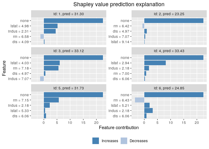
The following example shows how a simple xgboost model is trained using the Boston Housing Data, and how shapr explains the individual predictions.

library(xgboost)
library(shapr)

data("Boston", package = "MASS")

x_var <- c("lstat", "rm", "dis", "indus")
y_var <- "medv"

ind_x_test <- 1:6
x_train <- as.matrix(Boston[-ind_x_test, x_var])
y_train <- Boston[-ind_x_test, y_var]
x_test <- as.matrix(Boston[ind_x_test, x_var])

# Looking at the dependence between the features
cor(x_train)
#>            lstat         rm        dis      indus
#> lstat  1.0000000 -0.6108040 -0.4928126  0.5986263
#> rm    -0.6108040  1.0000000  0.1999130 -0.3870571
#> dis   -0.4928126  0.1999130  1.0000000 -0.7060903
#> indus  0.5986263 -0.3870571 -0.7060903  1.0000000

# Fitting a basic xgboost model to the training data
model <- xgboost(
  data = x_train,
  label = y_train,
  nround = 20,
  verbose = FALSE
)

# Prepare the data for explanation
explainer <- shapr(x_train, model)
#> The specified model provides feature classes that are NA. The classes of data are taken as the truth.

# Specifying the phi_0, i.e. the expected prediction without any features
p <- mean(y_train)

# Computing the actual Shapley values with kernelSHAP accounting for feature dependence using
# the empirical (conditional) distribution approach with bandwidth parameter sigma = 0.1 (default)
explanation <- explain(
  x_test,
  approach = "empirical",
  explainer = explainer,
  prediction_zero = p
)

# Printing the Shapley values for the test data.
# For more information about the interpretation of the values in the table, see ?shapr::explain.
print(explanation$dt)
#>      none     lstat         rm       dis      indus
#> 1: 22.446 5.2632030 -1.2526613 0.2920444  4.5528644
#> 2: 22.446 0.1671903 -0.7088405 0.9689007  0.3786871
#> 3: 22.446 5.9888016  5.5450861 0.5660136 -1.4304350
#> 4: 22.446 8.2142203  0.7507569 0.1893368  1.8298305
#> 5: 22.446 0.5059890  5.6875106 0.8432240  2.2471152
#> 6: 22.446 1.9929674 -3.6001959 0.8601984  3.1510530

# Finally we plot the resulting explanations
plot(explanation)

Contribution

All feedback and suggestions are very welcome. Details on how to contribute can be found here. If you have any questions or comments, feel free to open an issue here.

Please note that the ‘shapr’ project is released with a Contributor Code of Conduct. By contributing to this project, you agree to abide by its terms.

References