simlandr:
Simulation-Based Landscape Construction for Dynamical Systems

simlandr:
Simulation-Based Landscape Construction for Dynamical Systems

A toolbox for constructing potential landscapes for dynamical systems using Monte Carlo simulation. The method is based on the potential landscape definition by Wang et al. (2008) (also see Zhou & Li, 2016, for further mathematical discussions) and can be used for a large variety of models.
simlandr can help to:
hash_big.matrix class, and perform out-of-memory
calculation;You can install the development version from GitHub with:
install.packages("devtools")
devtools::install_github("Sciurus365/simlandr")
devtools::install_github("Sciurus365/simlandr", build_vignettes = TRUE) # Use this command if you want to build vignetteslibrary(simlandr)
# Simulation
## Single simulation
single_output_grad <- sim_fun_grad(length = 1e4, seed = 1614)
## Batch simulation: simulate a set of models with different parameter values
batch_arg_set_grad <- new_arg_set()
batch_arg_set_grad <- batch_arg_set_grad %>%
add_arg_ele(
arg_name = "parameter", ele_name = "a",
start = -6, end = -1, by = 1
)
batch_grid_grad <- make_arg_grid(batch_arg_set_grad)
batch_output_grad <- batch_simulation(batch_grid_grad, sim_fun_grad,
default_list = list(
initial = list(x = 0, y = 0),
parameter = list(a = -4, b = 0, c = 0, sigmasq = 1)
),
length = 1e4,
seed = 1614,
bigmemory = FALSE
)
batch_output_grad
#> Output(s) from 6 simulations.
# Construct landscapes
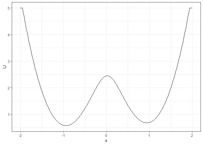
## Example 1. 2D landscape
l_single_grad_2d <- make_2d_static(single_output_grad,
x = "x",
from = -2, to = 2, adjust = 2
)
plot(l_single_grad_2d)
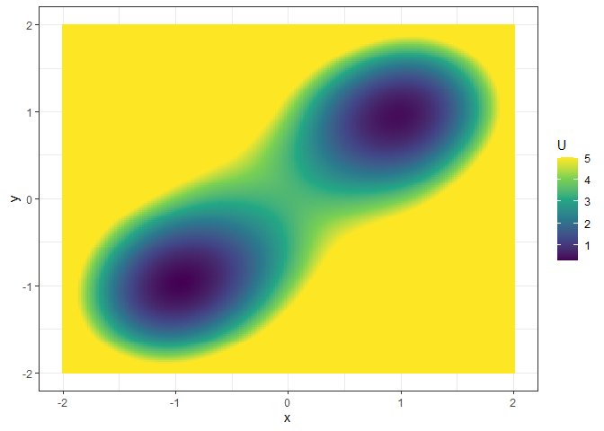
## Example 2. 3D (x, y, color) plot matrix with two varying parameters
l_single_grad_3d <- make_3d_static(single_output_grad,
  x = "x", y = "y",
  lims = c(-2, 2, -2, 2), h = 0.05,
  kde_fun = "ks"
)
#> Calculating the smooth distribution...
#> Done!
#> Making the plot...
#> Done!
#> Making the 2d plot...
#> Done!
plot(l_single_grad_3d, 2)
# Calculate energy barriers
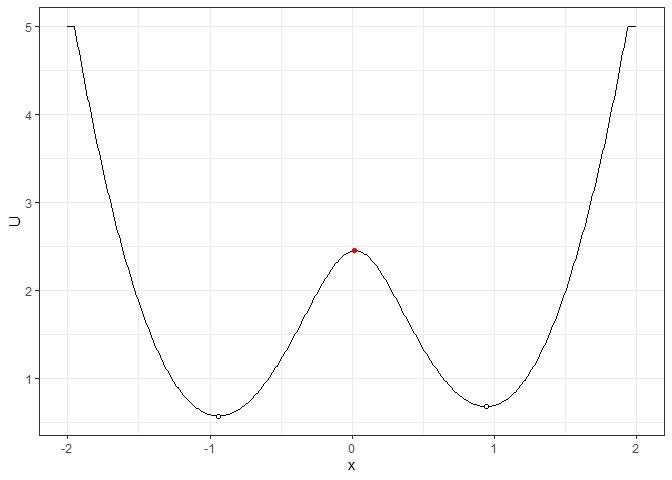
## Example 1. Energy barrier for the 2D landscape
b_single_grad_2d <- calculate_barrier(l_single_grad_2d,
  start_location_value = -1, end_location_value = 1,
  start_r = 0.3, end_r = 0.3
)
get_barrier_height(b_single_grad_2d)
#> delta_U_start   delta_U_end
#>      1.877958      1.771488

plot(l_single_grad_2d) + get_geom(b_single_grad_2d)
## Example 2. Energy barrier for the 3D landscape
b_single_grad_3d <- calculate_barrier(l_single_grad_3d,
  start_location_value = c(-1, -1), end_location_value = c(1, 1),
  start_r = 0.3, end_r = 0.3
)
get_barrier_height(b_single_grad_3d)
#> delta_U_start   delta_U_end
#>      3.182738      3.080433
plot(l_single_grad_3d, 2) + get_geom(b_single_grad_3d)
See the vignettes of this package
(browseVignettes("simlandr") or https://psyarxiv.com/pzva3/) for more examples and
explanations.