The goal of tidysmd is to easily create tidy data frames of SMDs. tidysmd wraps the smd package to easily calculate SMDs across many variables and using several weights in order to easily compare different adjustment strategies.
You can install the most recent version of tidysmd from CRAN with:
install.packages("tidysmd")Alternatively, you can install the development version of tidysmd from GitHub with:
# install.packages("devtools")
devtools::install_github("malcolmbarrett/tidysmd")tidy_smd() supports both unweighted SMDs and weighted
SMDs.
library(tidysmd)
tidy_smd(nhefs_weights, c(age, education, race), .group = qsmk)
#> # A tibble: 3 × 4
#>   variable  weights    qsmk     smd
#>   <chr>     <chr>      <chr>  <dbl>
#> 1 age       unweighted 1     -0.282
#> 2 education unweighted 1      0.196
#> 3 race      unweighted 1      0.177
nhefs_weights contains several types of propensity score
weights for which we can calculate SMDs. Unweighted SMDs are also
included by default.
tidy_smd(
  nhefs_weights,
  c(age, race, education),
  .group = qsmk,
  .wts = c(w_ate, w_att, w_atm)
)
#> # A tibble: 12 × 4
#>    variable  weights    qsmk       smd
#>    <chr>     <chr>      <chr>    <dbl>
#>  1 age       unweighted 1     -0.282
#>  2 race      unweighted 1      0.177
#>  3 education unweighted 1      0.196
#>  4 age       w_ate      1     -0.00585
#>  5 race      w_ate      1      0.00664
#>  6 education w_ate      1      0.0347
#>  7 age       w_att      1     -0.0120
#>  8 race      w_att      1      0.00365
#>  9 education w_att      1      0.0267
#> 10 age       w_atm      1     -0.00184
#> 11 race      w_atm      1      0.00113
#> 12 education w_atm      1      0.00934
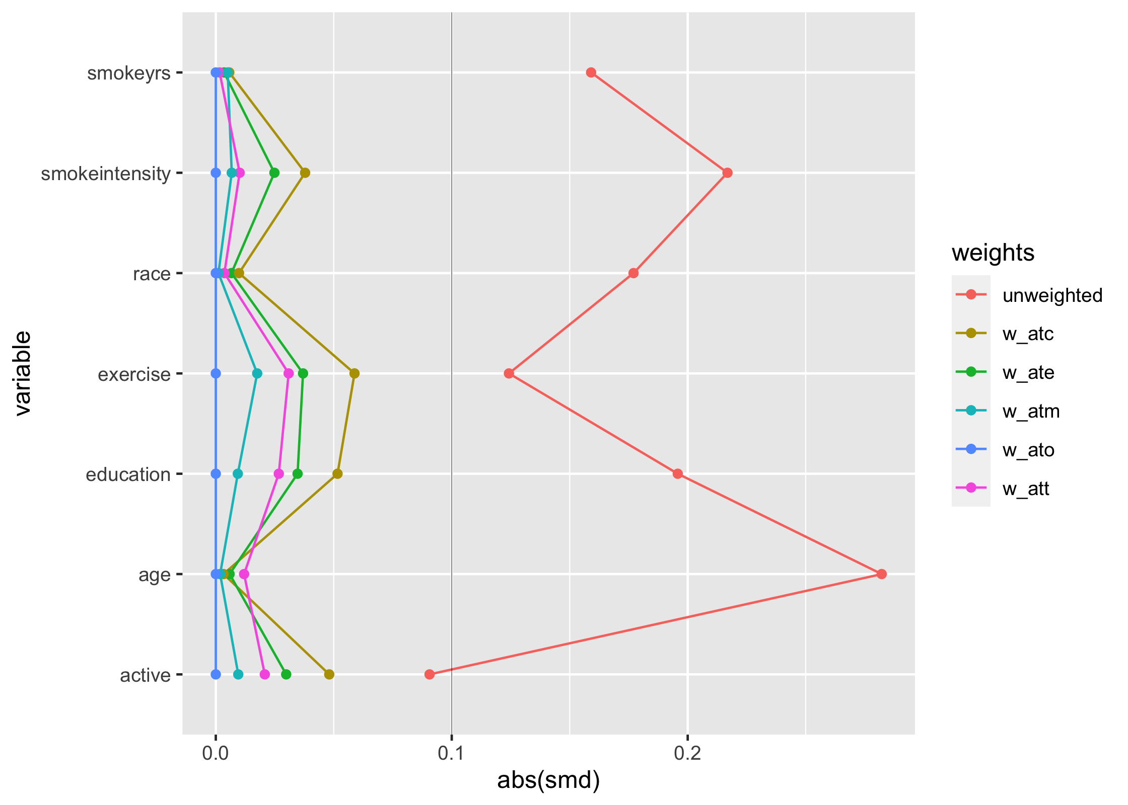
Having SMDs in a tidy format makes it easy to work with the estimates, for instance in creating Love plots:
library(ggplot2)
plot_df <- tidy_smd(
  nhefs_weights,
  race:active,
  .group = qsmk,
  .wts = starts_with("w_")
)

ggplot(
  data = plot_df,
  mapping = aes(x = abs(smd), y = variable, group = weights, color = weights)
) +
  geom_line(orientation = "y") +
  geom_point() +
  geom_vline(xintercept = 0.1, color = "black", size = 0.1)