This package presents the White’s Test of Heterocedasticity and a bootstrapped version of it, developed under the methodology of Jeong, J., Lee, K. (1999) (see references for further details).
You can install the development version from GitHub with:
This is an example which shows you how you can use the white_test and white_test_boot functions:
library(whitestrap)
#>
#> Please cite as:
#> Lopez, J. (2020), White's test and Bootstrapped White's test under the methodology of Jeong, J., Lee, K. (1999) package version 0.0.1

set.seed(123)
# Let's simulate some heteroscedastic data
n <- 100
y <- 1:n
sd <- runif(n, min = 0, max = 4)
error <- rnorm(n, 0, sd*y)
X <- y + error
df <- data.frame(y, X)
# OLS model
fit <- lm(y ~ X, data = df)
# White's test and Bootstrapped White's test
white_test(fit)
#> White's test results
#>
#> Null hypothesis: Homoskedasticity of the residuals
#> Alternative hypothesis: Heteroskedasticity of the residuals
#> Test Statistic: 12.88
#> P-value: 0.001597
white_test_boot(fit)
#> Bootstrapped White's test results
#>
#> Null hypothesis: Homoskedasticity of the residuals
#> Alternative hypothesis: Heteroskedasticity of the residuals
#> Number of bootstrap samples: 1000
#> Boostrapped Test Statistic: 12.88
#> P-value: 0.003In either case, the returned object is a list with the value of the statistical test and the p-value of the test. For the bootstrapped version, the number of bootstrap samples is also provided.
names(white_test(fit))
#> [1] "w_stat"  "p_value"
names(white_test_boot(fit))
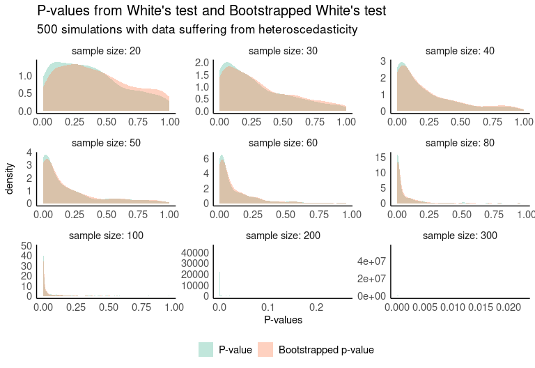
#> [1] "w_stat" "p_value" "iters"One way to compare the results of both tests is through simulations. The following plot shows the distribution of 500 simulations where the p-value of both tests is computed. The data used for this purpose were artificially generated to be heterocedastic, so low p-values are desirable.

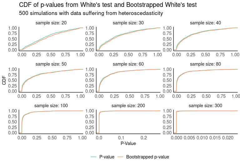
If we look at the cumulative distribution functions of both p-value distributions, we see that in small samples the bootstrapped test returns smaller p-values with higher probability.

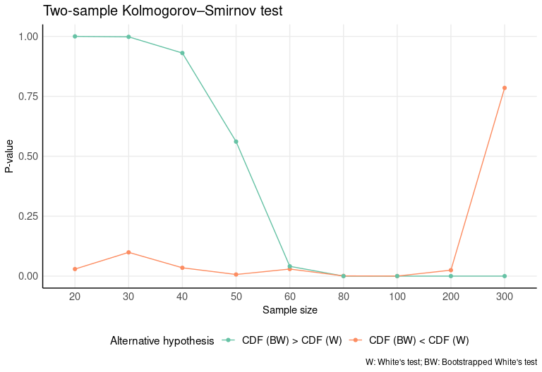
In order to check for differences between the two distributions, a two-sample Kolmogorov–Smirnov test is run. In this case, we’ll test whether one distribution stochastically dominates another, so the test will be run for both alternative sides (CDF (BW) > CDF (W) and CDF (BW) < CDF (W)). We see from the results that CDF (BW) statistically outperforms CDF (W) for samples < 60. No differences are appreciated with samples greater than or equal to 60.

Jeong, J., & Lee, K. (1999). Bootstrapped White’s test for heteroskedasticity in regression models. Economics Letters, 63(3), 261-267.
White, H. (1980). A Heteroskedasticity-Consistent Covariance Matrix Estimator and a Direct Test for Heteroskedasticity. Econometrica, 48(4), 817-838.
Wooldridge, Jeffrey M., 1960-. (2012). Introductory econometrics : a modern approach. Mason, Ohio, South-Western Cengage Learning.